Measures of Spread
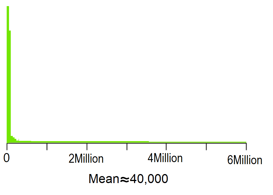
The median individual income in the US in 2019 was about $\small{\$}$40,000. While that tells us something about how much money people in the US are earning, by itself it doesn't tell us a great deal. To illustrate, if every individual in the US had an income of $\small{\$}$40,000, then $\small{\$40,000}$ would be the median. But the median would also be $\small{\$}$40,000 if half of individuals annual incomes of $\small{\$}$0 and the other half brought in $\small{\$}$80,000 annually. The distribution of annual income in the US is dramatically right skewed. To get a better understanding of what the distribution looks like, graphical summaries are helpful and numerical summaries describing how spread out the data are can add to our understanding.


Variance
The variance is a measure of how spread out the data values are around the mean. Since it describes spread in relation to the mean, the variance should always be used in conjunction with the mean as a measure of center. Like the mean, the variance is strongly affected by outliers thus it is most appropriate to use the variance with symmetric data.
The variance is a mean of the squared deviations of the data points from the mean. The deviation of a point from the mean is the distance between them: ith deviation\(\small{ = X_i - \bar{X}}\).
Deviation from the mean: The distance between a data point and the mean of the data.
Click on the plot to create a dot plot. Click on an existing dot to clear all dots above that point. The applet displays the values of the mean and standard deviation. Check the 'show mean' box to see the mean and the deviations from the mean.
$S^2 = \frac{1}{n-1}\sum_{i=1}^n\left(X_i-\bar{X}\right)^2$
Percentiles and Quartiles
Percentiles are an effective way to describe the spread of data that may not be symmetric. A percentile indicates a point such that a specified percentage of the data is smaller. For instance, the 70th percentile is a value such that 70 percent of the data is less than it. Like the median (which is itself the 50th percentile), percentiles are not affected by outliers.
Percentile: The pth percentile, $T_p$ is the value such that p% of the data are smaller than it.
There various methods for computing percentiles. Let $T_p$ denote the pth percentile. $T_p$ could be defined to be the value such that p% of the data is less than it (denote this value $L_p$), or as the value such that p% of the data is less than or equal to it (denote this $E_p$). Given the numbers from 1 to 100, $L_p = 31$ and $E_p=30$. We will define the pth percentile, $T_p$ as a weighted average of these two values.
$T_p = \frac{p}{100} E_p + \frac{100-p}{100}L_p$
$E_{30} = 30$ and $L_{30} = 31$
$T_{30} = \frac{30}{100}E_{30}+\frac{70}{100}L_p = 0.3(30) + 0.7(31) = 30.7.$
Notice that using the above definition of a percentile, the 50th percentile, $T_{50}$ corresponds to the median.
$E_{30} = 500$ and $L_{30} = 51$
$T_{30} = \frac{50}{100}E_{50}+\frac{50}{100}L_p = 0.5(50)+0.5(51) = 50.5$.
Since there is an even number of values in the list, the median is the mean of the middle two numbers, 50 and 51.
Thus, $M = \frac{50+51}{2} = 50.5$.
Quantiles are equivalent to percentiles but written in decimal rather than percent form. Thus the pth percentile is the p/100th quantile. Deciles and
quartiles are alternative designations for specific percentiles. Deciles refer the the percentiles where p is a multiple of 10.
Quartiles divide the data into quarters.
The first or lower quartile is the 25th percentile, the second quartile or median is the 50th percentile, the 3rd or upper quartile is the 75th percentile and the
4th quartile corresponds to the maximum. The distance between the upper and lower quartiles is called the Interquartile Range (IQR). One method for identifying outliers
is to consider any value that is more than 1.5$\times$IQR above the upper quartile or below the lower quartile an outlier.
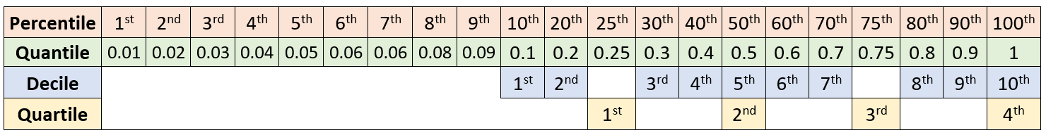
The table shows selected percentiles and quartiles of the 2020 net worth of US households.
