Chi-square Tests
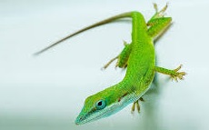
Researchers studying lizards investigated whether the color people wore affected how the lizards responded to them[1]. The researchers studied water anole lizards for which the orange is the sexually selected color. They dressed in orange, blue, or green while trying to capture the lizards and recorded the color worn and whether the capture attempt was successful.
In the study, the researchers wanted to determine if there was a relationship between two categorical variables. Hypothesis tests for categorical variables are referred to as
chi-square (usually pronounced "Kai square") tests because the test statistics involved have Chi-square distributions. Two types of chi-square tests are described
on this page.
The 'goodness-of-fit' test is used with one categorical variable to determine whether the distribution of counts in the different levels agrees with some
researcher-defined model. For example, this test could be used to determine whether a die is fair. The categorical variable of interest is the outcome of a roll, and observed
counts for the six categories would each be expected to be about 1/6 of the total if the die is fair.
The chi-square Test of Independence is used to determine whether there is a relationship between two categorical variables.
- A goodness-of-fit test that enables us to compare the proportions in multiple categories to hypothesized values and
- A test for independence that enables us to determine whether there is an association between two categorical variables.
The Chi-Square Goodness-of-Fit Test
A Goodness-of-Fit Test measures the discrepancy between observed cell counts and cell counts expected under the null hypothesis (according to the hypothesized distribution) to assess whether the hypothesized distribution is plausible.
According to the-numbers.com between 1995 and 2020, about 27% of movie revenue came from movies rated R, about 47% from movies rated PG-13, and 26% from movies with the other ratings (PG, G, NR, etc.). Do the movies available from Netflix reflect these proportions? That is, are 47% of Netflix offerings rated PG-13, 27% rated R, with the other ratings making up the remaining 26%?
Since this is a hypothesis test, we will consider each of the steps in the process as it relates to the goodness-of-fit test:
- State hypotheses.
- Collect data.
- Construct a test statistic
- Compute a p-value.
- Draw conclusions (in statistical terms and in context)
Step 1: State Hypotheses
For a goodness of fit test, the null hypothesis is that the observed proportions in each of k categories are equal to the hypothesized values.
The parameters of interest are the probabilities that an observation falls in each cell. $p_i$ denotes the true probability that an observation is in cell $i$ and
$p_i^*$ denotes the null value, or the probability expected under the null hypothesis.
The null hypothesis is that true proportions are equal to the hypothesized values.
$$H_0: p_1=p_1^*, p_2=p_2^*, \ldots ,p_k=p_k^* $$
The alternative hypothesis is that at least one of the true cell proportions is not equal to the hypothesized value.
$$H_A: p_i\neq p_i^* \texttt{ for some }i$$
Let $p_1$, $p_2$, and $p_3$ correspond to the groups with ratings R, PG-13, and everything else respectively. Using information provided previously:
$H_0:p_1=0.27$, $p_2=0.47$, $p_3=0.26$
$H_A: p_i\neq p_i^*$ for some $i$
Step 2: Collect Data
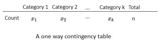
The data for a goodness of fit test are displayed in a one way contingency table. This is a table that displays the counts in different
levels of a single categorical variable.
Each of n observations can be classified into exactly one of k categories or cells in the table. The cell frequencies are denoted $x_1, x_2, \dots x_k$. $x_1+x_2+ \cdots + x_k = n$.
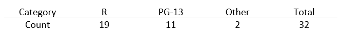
The data for the Netflix movie ratings example are shown in the table.
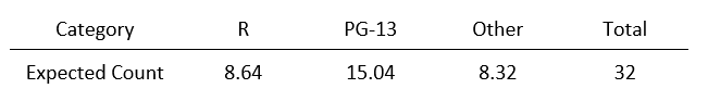
If the null hypothesis is true, that is $p_1=p_1^*$, $p_2=p_2^*$, ... , $p_k=p_k^*$ and the total number of observations is $n$, then we would expect to see $p_i^*\cdot n$ observations in cell $i$. We denote the expected count for cell i as $e_i$.
Note: $e_1+ e_2+ \dots+e_k=n$.
Warning: For the test to be valid, each of the expected counts should be at least 5.
\(\begin{array}{rcl} e_1 & = & 0.27\times 32 & = & 8.64\\ e_2 & = & 0.47\times 32 & = & 15.04\\ e_3 & = & 0.26\times 32 & = & 8.32 \end{array}\)
The test statistics for the goodness-of-fit test facilitates comparison of the observed and expected counts.
$X^2=\sum_{i=1}^n \frac{(x_i-e_i)^2}{e_i} \sim \chi^2_{k-1}$.
That is $X^2=\sum_{\texttt{(all cells)}} \frac{(\texttt{ith observed value} - \texttt{ith expected value})^2}{\texttt{ith expected value}}$
The statistic has a chi-square distribution with $k-1$ degrees of freedom (the number of categories minus 1).
The test statistic for the movie rating goodness-of-fit test is
$$X^2 = \frac{(19-8.64)^2}{8.64}+\frac{(11-15.04)^2}{15.04}+\frac{(2-8.32)^2}{8.32} = 18.308$$
Compute a p-value
The p-value is for this test comes from the right tail of a $\chi^2_{k-1}$ distribution.
$ p-value= P(\chi^2 > X^2)$
$P(\chi^2_2 > X^2) = P(\chi^2_2 > 18.308) = 0.0001$
Draw Conclusions
As with previous tests, we must draw conclusions statistically (that is, reject or fail to reject the null hypothesis) and in context. If we reject the null hypothesis, we conclude that the probabilities stated in the null hypothesis do not fit the data.The p-value for the movie rating goodness-of-fit test is 0.0001 which is much smaller than the usual signficance level of $0.05$, thus we reject the null hypothesis. The results are highly statistically significant.
There is strong evidence that the proportions of Netflix movies in the various ratings categories do not reflect the proportions of movie revenue generate by movies in these ratings categories.
The Chi-square Test of Independence
A chi-square test of independence is used to determine whether two variables are independent.Researchers studying lizards investigated whether the color people wore affected how the lizards responded to them[1]. The researchers studied water anole lizards for which the orange is the sexually selected color. They dressed in orange, blue, or green while trying to capture the lizards and recorded the color worn and whether the capture attempt was successful.
For a test of independence, the null hypothesis is that the variables are independent of each other, the alternative hypothesis is that they are not.
$H_0$: Lizard capture is independent of color worn by researcher.
$H_A$: Lizard capture is not independent of color worn by researcher.
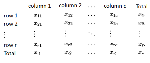
The data for a goodness of fit test are displayed in a two way contingency table. This is a table in which the cell counts indicate how many observations
were classified in the corresponding row and column categories.
If the first category has $r$ levels and the second has $c$ levels $1 \leq i \leq r$ and $1 \leq j \leq c$, then $x_{i,j}$ is the
in the $i$th row and $j$th column of the table.
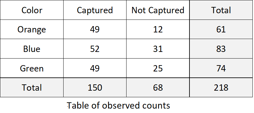
A two-way contingency table for the lizard/color data:
Step 3: Construct a Test Statistic
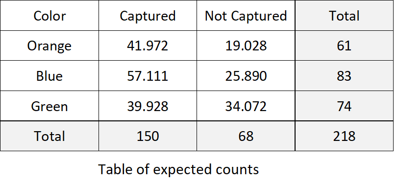
The null hypothesis for the test of independence is that the row and column variables are independent of one another. Under this hypothesis, the expected count for the $i$th row and $j$th column of the table is $e_{ij} = \frac{x_{r\cdot}x_{\cdot c}}{x_{\cdot\cdot}} = \frac{\texttt{(row i total)}\texttt{(column j total)}}{\texttt{(grand total)}}.$
Warning: For the test to be valid, each of the expected counts should be at least 5.
\(\begin{array}{ccccccccccc} e_{11} & = & \frac{61\cdot 150}{218} & = & 41.972 & & e_{12} & = & \frac{61\cdot 68}{218} & = & 13.028\\ e_{21} & = & \frac{83\cdot 150}{218} & = & 57.110 & & e_{22} & = &\frac{83\cdot 68}{218} & = & 25.890\\ e_{31} & = & \frac{74\cdot 150}{218} & = & 39.928 & & e_{32} & = & \frac{74\cdot 68}{218} & = & 34.072 \end{array}\)
The test statistic of the test of independence is very similar to that of the goodness-of-fit test. It is found by summing over all cells the squared difference between the observed and expected counts divided by the expected count.
$X^2=\sum_{ij}n \frac{(x_{ij}-e_{ij})^2}{e_{ij}} \sim \chi^2_{(r-1)(c-1)}$.
That is $X^2=\sum_{\texttt{(all cells)}} \frac{(\texttt{ijth observed value} - \texttt{ijth expected value})^2}{\texttt{ijth expected value}}$
The statistic has a chi-square distribution with $(r-1)(c-1)$ degrees of freedom (the number of row minus 1 times the number of columns minus 1).
The test statistic lizard/color test of independence is
$$\small{\begin{array}{ccccc} X^2 & = & \frac{(49-41.97)^2}{41.97} & + & \frac{(12-19.028)^2}{19.028} & + & \frac{(52-57.11)^2}{57.11}\\ & + & \frac{(31-25.890)^2}{25.890} & + & \frac{(49-39.928)^2}{39.928} & + & \frac{(25-34.072)^2}{34.072} \\ & = & 9.692 & & & &\end{array}}$$
Compute a p-value
The p-value for the test of independence comes from the right tail of a chi-square distribution.$P(\chi^2_2 > X^2) = P(\chi^2_2 > 9.692) = 0.008$
Draw Conclusions
As with previous tests, we must draw conclusions statistically (that is, reject or fail to reject the null hypothesis) and in context. If we reject the null hypothesis, we conclude that the variables are not independent.The p-value for the lizard/color test of independence is 0.008 which is much smaller than the usual signficance level of $0.05$, thus we reject the null hypothesis. The results are highly statistically significant.
There is evidence that the success of a capture and the color the researcher was wearing are not independent.
Is being family friendly (rated G or PG) independent of whether a movie is short (less than 90 minutes)?
To answer this question, we'll conduct a chi-square test of independence.
The hypotheses for the test are:
- $H_0$: family friendly and short are independent.
- $H_A$: family friendly and short are not independent.
 The expected counts are:
$$\small{\begin{array}{ccccc} e_{11} & = & \frac{23\times 28}{79}& = & 8.15\\
e_{12} & = & \frac{23\times 51}{79} & = & 14.85\\
e_{21} & = & \frac{56\times 28}{79} & = & 18.85\\
e_{22} & = & \frac{56\times 51}{79} & = & 36.15\end{array}}$$
Which give a test statistic of
$$\small{\begin{array}{rcl} X^2 & = & \frac{(18-8.15)^2}{8.15}+\frac{(5-14.85)^2}{14.85}+\frac{(10-18.85)^2}{18.85}+\frac{(46-36.15)^2}{36.15}\\
& = & 25.277\end{array}}$$
The expected counts are:
$$\small{\begin{array}{ccccc} e_{11} & = & \frac{23\times 28}{79}& = & 8.15\\
e_{12} & = & \frac{23\times 51}{79} & = & 14.85\\
e_{21} & = & \frac{56\times 28}{79} & = & 18.85\\
e_{22} & = & \frac{56\times 51}{79} & = & 36.15\end{array}}$$
Which give a test statistic of
$$\small{\begin{array}{rcl} X^2 & = & \frac{(18-8.15)^2}{8.15}+\frac{(5-14.85)^2}{14.85}+\frac{(10-18.85)^2}{18.85}+\frac{(46-36.15)^2}{36.15}\\
& = & 25.277\end{array}}$$Notice that all of the expected counts are larger than 5 so use of the chi-square distribution is reasonable.
The pvalue for the test is $P(\chi^2_1 > 25.277) = 4.97\times 10^{-7}$.
Since the p-value is less than 0.05, it is unlikely that these data would occur by chance if family friendly and short were independent. We reject the null hypothesis and conclude that the variables are not independent.