Confidence Intervals

On Memorial Day, 2020, Netflix had 834 movies in its library. An estimate of the mean run time of these movies, based on a sample of size 32 is 104.5 minutes with a standard error of 3.2 minutes. A 95% confidence interval for the mean run time of all 834 movies available on that date is (98, 111) minutes.

Illustration of a person’s hands holding a black and white movie clapperboard against a solid pink background.

A $(1-\alpha)100\%$ confidence interval gives a set of plausible values for a parameter. It is formed from the point estimate and a margin of error associated with a particular level of confidence.

Confidence intervals that are based on symmetric distributions such as the normal or t distributions usually have the same basic form: point estimate $\pm$ the margin of error.

The margin of error is determined by the standard error and a desired level of confidence.

Many confidence intervals have the form point estimate $\pm$ the margin of error.

Example: A 95% Confidence Interval for Movie Run Time

A 95% confidence interval for the mean runtime of Netflix movies is (98, 111). The point estimate obtained from the sample is $\bar{X}=104.5$ minutes and the margin of error is 6.5 minutes. $104.5\pm 6.5: (98, 111)$

The confidence level $(1-\alpha)100\%$ indicates the probability that the interval will cover the parameter of interest. The most common confidence level is 95% in which case $\alpha=0.05$: $(1-0.05)100\% = 95\%$. 90% and 99% are also common confidence levels but the level can be anything the researcher chooses. 100% confidence levels are possible but usually not at all useful. We'll discuss this further when we talk about interpretation below.

The Confidence level, $(1-\alpha)100\%$, specifies the probability that the confidence interval covers the true parameter value.

Constructing Confidence Intervals

A confidence interval for a mean has the form introduced previously: point estimate $\pm$ the margin of error. The margin of error itself is composed of a critical value that gives the desired confidence level, and the standard error thus the general form of the confidence interval can be re-written as: $$\text{point estimate }\pm \text{(critical value)}\times\text{(standard error)}$$

Point Estimate

The point estimate is the observed value of the statistic computed from the data. To construct a confidence interval for $\mu$, the point estimate is the observed value of the sample mean, $\bar{x}$. Note that the lowercase x indicates that this is an observed value rather than a random variable.

Example: A 95% Confidence Interval for Movie Run Time

The point estimate for the mean runtime of movies available from Netflix, $\mu$, was computed from a random sample of 32 movies. The data are shown here.

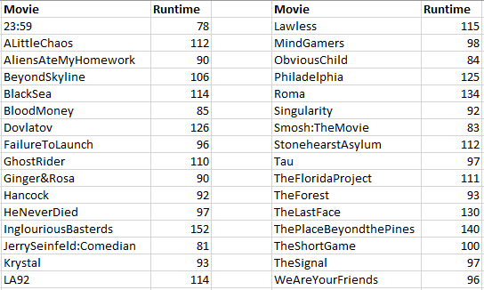
A two-column table listing movies and their runtimes. The left column includes films such as “23:59” (78 minutes), “ALittleChaos” (112), “InglouriousBasterds” (152), and “LA92” (114). The right column continues with movies like “Lawless” (115), “Roma” (134), “ThePlaceBeyondthePines” (140), and “WeAreYourFriends” (96). The runtimes range from 78 to 152 minutes.

A two-column table listing movies and their runtimes. The left column includes films such as “23:59” (78 minutes), “ALittleChaos” (112), “InglouriousBasterds” (152), and “LA92” (114). The right column continues with movies like “Lawless” (115), “Roma” (134), “ThePlaceBeyondthePines” (140), and “WeAreYourFriends” (96). The runtimes range from 78 to 152 minutes.

The point estimate for the mean runtime is $\bar{x} = 104.5$ minutes.

Critical Values

A critical value indicates how many standard errors either side of the mean a confidence interval must extend in order to obtain the desired level of confidence. It's value depends on the distribution of the relevant statistic.

When computing a confidence interval for a population mean, the relevant statistic is the standardized sample mean, $\frac{\bar{X}-\mu}{s.e.(\bar{X})}$.

In the discussion of sampling distributions we learned that the distribution of this standarized statistic depends on the population distribution and whether the population variance is known.

If the population is normally distributed and $\sigma^2$ is known $\frac{\bar{X}-\mu}{s.e.(\bar{X})} = \frac{\bar{X}-\mu}{\sigma/\sqrt{n}} \sim N(0,1)$
If the population is not normally distributed, but the sample size is large:
1. If $\sigma^2$ is known $\frac{\bar{X}-\mu}{s.e.(\bar{X})} = \frac{\bar{X}-\mu}{\sigma/\sqrt{n}} \sim N(0,1)$.
2. If $\sigma^2$ is unknown $\frac{\bar{X}-\mu}{s.e.(\bar{X})} \approx \frac{\bar{X}-\mu}{S/\sqrt{n}} \stackrel{\boldsymbol{\cdot}}{\sim} N(0,1)$.
If the population is normally distributed, $\sigma^2$ is unknown, $\frac{\bar{X}-\mu}{s.e.(\bar{X})} \approx \frac{\bar{X}-\mu}{S/\sqrt(n)} \sim t_{n-1}$

In most cases, the population variance is not known. If the distribution of the population is approximately normal, the t-distribution will be useful regardless of the sample size (as the sample size increases, $t\rightarrow N(0,1)$). However, if the population distribution is very different from normal, the Central Limit Theorem indicates that the distribution of $\frac{\bar{X}-\mu}{S/\sqrt{n}}$ will be approximately standard normal if the sample size is large enough.

A critical value is a point under a distribution that marks a cut-off corresponding to a region with specified probability.

We denote a critical value as $z_{\alpha}$ if $\frac{\bar{X}-\mu}{s.e.(\bar{X})}\sim N(0,1)$ and $t_{\alpha,\nu}$ if $\frac{\bar{X}-\mu}{s.e.(\bar{X})}\sim t_{\nu}$ where $\alpha$ is the area to the right of the critical value under the relevant distribution. For our purposes, we'll usually think about $Z_\frac{\alpha}{2}$ rather than $Z_{\alpha}$. If we construct a two-sided $(1-\alpha)100\%$ confidence interval (one-sided intervals exist but are not as widely used), then $\alpha$ is the probability that the interval does not cover the parameter and half of this area should be on either end of the interval.

Normal Distribution Critical Values

In the standard normal curve shown, the area to the right of $z_{\frac{\alpha}{2}}$ is $\frac{\alpha}{2}$. Since the curve is symmetric around 0, the area to the left of $-z_{\frac{\alpha}{2}}$ is also $\frac{\alpha}{2}$, that means that the area between those two points is $1-(2\cdot\frac{\alpha}{2}) = 1 - \alpha$.

Drag the triangle at $Z_{\frac{\alpha}{2}}$ to see how these values change.

t Distribution Critical Values

In the $t_{\nu}$ curve shown, the area to the right of $t_{\frac{\alpha}{2},\nu}$ is $\frac{\alpha}{2}$. Since the curve is symmetric around 0, the area to the left of $-t_{\frac{\alpha}{2},\nu}$ is also $\frac{\alpha}{2}$, that means that the area between those two points is $1-(2\cdot\frac{\alpha}{2}) = 1 - \alpha$.

Drag the triangle at $t_{\frac{\alpha}{2}, \nu}$ and use the slider to adjust the degrees of freedom to see how these values change.

Example: Critical Values

The population standard deviation, that is, the standard deviation of the runtime of all Netflix movies, is unknown but our sample size is large enough that, from the Central Limit Theorem, we would expect the distribution of the sample mean to be approximately normal so we will use the normal distribution to obtain a critical value. Since 95% is the most common confidence level, we will find the critical value for constructing a 95% confidence interval.

For a 95% confidence interval, $\alpha = 1-0.95 = 0.05$, thus $\frac{\alpha}{2} = 0.025$. Using the 'Normal Critical Values' applet above, we find that when $\frac{\alpha}{2} = 0.025$, $z_{\frac{\alpha}{2}}=1.96$.

$A normal distribution curve labeled N(0,1) representing a standard normal distribution. The middle 95% of the area under the curve is shaded between −1.96 and 1.96, marked as (1 - \alpha = 0.95). The two tails each have an area of 0.025 labeled (\alpha/2 = 0.025), with the corresponding z-scores (z_{-\alpha/2} = -1.96) and (z_{\alpha/2} = 1.96).$

Standard Error

We know from previous discussions that if a sample is drawn from a population with variance $\sigma^2$ then the standard error of $\bar{X}$ is $\frac{\sigma}{\sqrt{n}}$. Since $\sigma^2$ is generally unknown, we typically replace it with the estimated standard error $\frac{S}{\sqrt{n}}$.

Example: Compute the standard error needed to contruct a confidence interval for the mean runtime of Netflix movies. Since $\sigma$, the population standard deviation, is unknown we will use S, the sample standard deviation to find the estimated standard error of $\bar{X}$.

From the data we find that $s = 18.22$. Since the sample size is 32, estimated s.e.$(\bar{X}) = \frac{18.22}{\sqrt{32}}=3.22$.

Putting It Together

A confidence interval for a population mean $\mu$ has the form: $$\text{point estimate }\pm \text{(critical value)}\times\text{(standard error)}$$

When the distribution of the population is approximately normal, the critical value can be obtained from a t-distribution so the $(1-\alpha)100\%$ confidence interval is $$\left(\bar{x} - t_{\frac{\alpha}{2},\nu}\frac{s}{\sqrt{n}}, \bar{x} + t_{\frac{\alpha}{2},\nu}\frac{s}{\sqrt{n}}\right)$$
If the population distribution is not normal, but the sample size is large (around 30 is typically large enough) then the Central Limit Theorem justifies us in using the standard normal distribution to obtain the critical values thus the form of a $(1-\alpha)100\%$ confidence interval for $\mu$ is $$\left(\bar{x} -z_{\frac{\alpha}{2}}\cdot \frac{s}{\sqrt(n)}, \bar{x} +z_{\frac{\alpha}{2}}\cdot \frac{s}{\sqrt(n)}\right)$$
Note that, when the sample size is large, the critical values from a t-distribution will be approximately equal to those from a normal distribution. Thus, in practice, the t-distribution is often used in both of the above cases to construct confidence intervals for a mean.

From the definition of a critical value, $P(-t_{\alpha/2}\leq T \leq t_{\alpha/2}) = 1 - \alpha$ where $T\sim t_{n-1}$. Thus, since $\frac{\bar{X}-\mu}{s/\sqrt{n}}\sim t_{n-1}$, $P(-t_{\alpha/2}\leq \frac{\bar{X}-\mu}{s/\sqrt{n}} \leq t_{\alpha/2}) = 1-\alpha$. The form of the confidence interval, comes from solving this inequality for $\mu$.

$\begin{array}{rcl} 1 - \alpha &=& P(-t_{\alpha/2} &\leq& \frac{\bar{X}-\mu}{s/\sqrt{n}} &\leq& t_{\alpha/2}) \\ &=& P(-t_{\alpha/2}\cdot \frac{s}{\sqrt(n)} &\leq& \bar{X}-\mu &\leq& t_{\alpha/2}\cdot \frac{s}{\sqrt{n}}) \\ &=& P(-\bar{X} -t_{\alpha/2}\cdot \frac{s}{\sqrt{n}} &\leq& -\mu &\leq& -\bar{X} + t_{\alpha/2}\cdot \frac{s}{\sqrt{n}})\\ &=& P(\bar{X} -t_{\alpha/2}\cdot \frac{s}{\sqrt{n})} &\leq& \mu &\leq& \bar{X} + t_{\alpha/2}\cdot \frac{s}{\sqrt{n}}) \end{array}$

The form of the other confidence intervals discussed in this section can be derived in a similar fashion.

Example: Milk Protein

For a sample of 10 cows that had recently given birth, the mean protein content in 40oz of milk was 3.4g with a sample standard deviation of 0.4 g. Find a 95% confidence interval for the mean protein content of the milk.

Since the sample is small, use the t-distribution to obtain the critical value for the confidence interval. For a 95% confidence interval, $(1-\alpha)\cdot 100\% = 95\%$, so $\alpha = 0.05$ and $\alpha/2 = 0.025$

$\bar{x} = 3.4$
$s = 0.4$
$t_{0.025,9} = 2.26$
95% CI: $(3.4 - 2.26\cdot \frac{0.4}{\sqrt{10}}, 3.4 + 2.26\cdot \frac{0.4}{\sqrt{40}}) = (3.114, 3.686)$.

Example: Netflix Movies

On Memorial Day, 2020, Netflix had 834 movies in its library. A point estimate for the mean run time of these movies, based on a sample of size 32 is 104.5 minutes with a standard error of 3.2 minutes. Show that a 95% CI for the mean runtime of the Netflix movies is (97,111).

For a 95% confidence interval, $(1-\alpha)\cdot 100\% = 95\%$, so $\alpha = 0.05$ and $\alpha/2 = 0.025$

Since the sample size is larger than 30 and the population standard deviation is unknown, we'll use the normal distribution to obtain critical values.
$\bar{x} = 104.5$
$s.e.(\bar{X}) = \frac{s}{\sqrt{32}} = 3.2$
$z_{0.025} = 1.96$
95% CI (rounded to the nearest minute): $(104.5 - 1.96\cdot 3.2, 104.5 + 1.96\cdot 3.2) = (98, 111)$.

Note: Since the t-distribution converges to the normal distribution as the sample size increases, using critical values from the t-distribution yields a similar result.
$t_{0.025,31} = 2.04$
95% CI (rounded to the nearest minute): $(104.5 - 2.04\cdot 3.2, 104.5 + 2.04\cdot 3.2) = (98, 111)$.

Confidence Intervals for a Proportion

As with confidence intervals for a mean, a confidence interval for a proportion, p, has this familiar form: $$\text{point estimate }\pm \text{(critical value)}\times\text{(standard error)}$$

Point Estimate

A point estimate for a population proportion, p, is the observed value of the sample proportion, $\hat{p}$.

Critical Values

The critical value for a confidence interval for a proportion comes from the normal distribution, that is $z_{\frac{\alpha}{2}}$.

The critical value depends on the distribution of the the standardized sample proportion: $\frac{\hat{p}-p}{\sqrt{\frac{p(1-p)}{n}}}$. The distribution of this standarized statistic is approximately standard normal when the sample size is large.

Standard Error

The standard error of $\hat{p}$ is $\sqrt{\frac{p(1-p)}{n}}$. Notice that this depends on the value of the parameter. Since $p$ is unknown (or it wouldn't need to be estimated), use $\hat{p}$ to find the estimated standard error: $\frac{\hat{p}-p}{\sqrt{\frac{\hat{p}(1-\hat{p})}{n}}}$.

Putting it Together

When the sample size is large, a $(1-\alpha)\cdot 100\%$ CI for a proportion is $\left(\hat{p}-z_{\alpha/2}\cdot \sqrt{\frac{\hat{p}(1-\hat{p})}{n}}, \hat{p}+z_{\alpha/2}\cdot \sqrt{\frac{\hat{p}(1-\hat{p})}{n}}\right)$.

A $(1-\alpha)100\%$ confidence interval for $p$ when n is large
$\left(\hat{p}-z_{\alpha/2}\cdot \sqrt{\frac{\hat{p}(1-\hat{p})}{n}}, \hat{p}+z_{\alpha/2}\cdot \sqrt{\frac{\hat{p}(1-\hat{p})}{n}}\right)$.

Example: Picture Yourself

In 2009, the camera company, Nikon, released the results of a survey called "Picture Yourself". For the survey, they obtained a sample of 1000 US adults. They found that the proportion of respondents said that they look better in person than they do in photographs was 0.79. Find a 90% confidence interval for the true proportion of US adults who think they look better in person than in photographs.

For a 90% confidence interval, $(1-\alpha)\cdot 100\% = 90\%$, so $\alpha = 0.1$ and $\alpha/2 = 0.05$

$\hat{p}=0.79$
$z_{0.05} = 1.65$
90% CI: $\left(0.79 - 1.65\cdot \sqrt{\frac{0.79(0.21)}{1000}},0.79 + 1.65\cdot \sqrt{\frac{0.79(0.21)}{1000}}\right) = (0.77, 0.81)$.

Interpreting Confidence Intervals

A confidence interval is a set of plausible values for the parameter of interest. From the derivation, we also saw that the confidence level gives the probability that the interval covers the parameter. It is typical to say "we are 95% confident that the interval covers the parameter" for a 95% confidence interval.

The applet below illustrates another way to think about confidence intervals. If the process of sampling and computing a CI were repeated 100 times, we'd expect that about 95 (99, 90, etc.) of the resulting 95% (99%, 90%, etc.) confidence intervals would cover the true parameter.

CI Applet

Use the applet to simulate drawing 100 samples from the jar of balls and computing a CI interval for the proportion of blue balls based on each sample.

Use the 'show p' checkbox to show the true proportion of blue balls. When this box is selected, the intervals that miss the parameter are colored red.

When the confidence level is set to 95, on average, 5 of the intervals will miss. Consider:

How does the confidence level affect the width of the confident interval? Try changing the confidence level in the applet, how do the intervals change?

How does the sample size affect the width of the confident interval? Try changing the sample size in the applet and generating a new set of intervals, how do these intervals compare?

Increasing the confidence level of a confidence interval widens the interval. When more values are admitted, there is a greater probability of that one of them is correct.

Increasing the confidence level results in wider confidence intervals.

Assuming the sample standard deviation remains the same, increasing the sample size results in a more narrow interval. The margin of error of a confidence interval is the product of the critical value and the standard error. The standard error, in turn, is the standard deviation divided by the sample size thus the larger the sample size, the smaller the standard error and the narrower the interval.

All else being equal, a larger sample size results in a narrower confidence interval.

Issues of Sample Size

Sometimes a researcher desires a certain level of precision in the confidence interval she constructs. For instance, she might like to have a confidence interval for the protein in milk that is no more than 0.1 grams wide. How large would the sample need to be to attain this?

Each confidence interval on this page has the same basic form: $\text{point estimate }\pm \text{margin of error}$. Since the margin of error is subtracted from the point estimate to get the lower endpoint of the interval and added to the point estimate to get the upper endpoint, the width, W, of the CI is twice the margin of error. That is $\small{W = 2\times \text{margin of error} = 2\times(\text{critical value})\times(\text{standard error})}$. It is possible to use this fact to find the sample size needed to obtain a certain level of precision in the interval.

$W = 2\times(\text{critical value})\times(\text{standard error})$

Example: Picture Yourself

In a survey of 1000 adults, 0.79 said they think they look better in person than in photographs. What sample size would we need to obtain a 95% confidence interval for the proportion of adults who think they look better in person than in photographs that is no longer than 0.02?

$W = 2\times(\text{critical value})\times(\text{standard error}) = 2\times z_{\frac{\alpha}{2}}\times\left(\sqrt{\frac{\hat{p}(1-\hat{p})}{n}}\right)$

$\hat{p} = 0.79$
$z_{0.025} = 1.96$
$s.e.(\hat{p}) = \sqrt{\frac{0.79(0.21)}{n}}$
Thus $0.02 = 1.96\cdot \sqrt{\frac{0.79(0.21)}{n}}$

Solving for $n$ we get $n=2048.5$. Since we're talking about sampling people, we'll round up to the nearest whole number. That is, we'd need a sample of size 2049 to obatain a 95% confidence interval that is no longer than 0.02.

Example: Milk Protein

For a sample of 10 cows that had recently given birth, the mean protein content in 40oz of milk was 3.4g with a sample standard deviation of 0.4 g. What sample size would we need to obtain a 95% confidence interval for the mean protein content that is 0.25g wide?

Solution:

$W = 2\times(\text{critical value})\times(\text{standard error}) = 2\times(t_{\frac{\alpha}{2},n-1})\times(\frac{s}{\sqrt{n}})$

Solving the equation for n gives $n = 4\left(\frac{t_{\alpha/2,n-1}S}{W}\right)^2$.

Notice that the critical value depends on $n$. As $n$ increases, the critical value decreases. In a previous prompt, we found that a sample size of 10 yielded a CI with width 0.42 thus the sample size must be greater than 10 and the corresponding critical value will be smaller than $t_{0.025,9} = 2.26$. So $n= 4\left(\frac{2.26(0.4)}{0.25}\right)^2 = 52.3$. A sample of size 53 is sufficient.