Inference for Two Means
Choosing a grocery store usually involves more than just prices. Store atmosphere, customer service, and location are a few criteria that might be important. However,
for most people, price is a concern. How would we use statistical methods to determine which of two local grocery stores is less expensive on average?
This question involves parameters from two populations - the mean price of items at each of the grocery stores. To addresses the question with inference, we must choose a random sample
from each population. Thus this is a "two-sample" problem.

A two-sample problem involves a comparison between two groups.
Comparing two groups (such as a treatment group to a control group or one treatment to another) to determine if the mean response differs is an important tool of research in many disciplines.
- Which of two brands of fertilizer results in the greater average yield from tomato plants?
- Is the mean body temperature of women is the same as that of men?
- On average, how much stronger is a person's dominant hand than their non-dominant hand?
Two-sample problems can involve either paired (related) samples or independent (unrelated) samples.
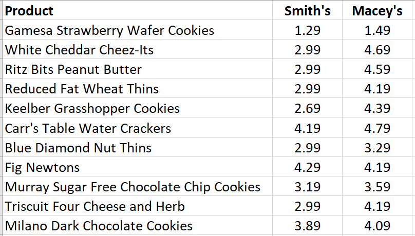
Which of two local grocery stores, Smith's or Macey's, has better prices on cookies and crackers? This question could be addressed using either paired or independent samples. If we take a a random sample of the cookie prices at each of the stores then the samples are independent. However, it makes sense to look at the same products at each store. We could choose a random sample of available cookies and crackers and look at the prices of those same products at each of the stores. In this case, the samples are paired.
Paired Samples
We analyze paired samples by reducing the problem to a one sample problem. Instead of comparing the first sample mean to the second, we consider the mean, $\mu_Z$, of the differences between the paired observations from the two sample and use a hypothesis test or a confidence interval to analze the results.
A Hypothesis Test for Paired Samples
Recall the Hypothesis Testing Process outlines previously:
- State hypotheses about the parameter.
- Collect data.
- Construct a test statistic.
- Compute a p-value.
- Draw conclusions (in statistical terms and in context).
Step 1: State Hypotheses
The null hypothesis for a test of paired samples has this form: $H_0: \mu_z = \delta$ where $\delta$ is the null value. Alternative hypotheses can be one or two sided, however, when comparing two samples the question of interest is often simply whether there is a difference between the groups. In this case, the null hypothesis is $H_0: \mu_z=0$ and the alternative hypothesis is $H_A:\mu_z\neq0$.
In comparing the cookie and cracker prices at two grocery stores, we want to know whether there is a difference in the mean prices. In other words, we're asking "is the difference 0 or not?". Thus the hypotheses for this test are: $$H_0: \mu_z=0 \texttt{ and } H_A:\mu_z\neq0.$$
Step 2: Collect Data
The data can be thought of as a random sample from one population matched with observations from a second population.
To collect data to compare the grocery stores, we chose a random sample from a complete list of the cookies and crackers available at one grocery store and then found the prices for those same products at the second grocery store. The data a shown here.
Denote the observations from the first sample as $x_1, x_2, \ldots x_n$ and those from the second sample as $y_1, y_2, \ldots y_n$. We calculate the differences between each of the pairs of observations $z_i = x_i-y_i$ for $i=1, 2, \ldots, n$, reducing the data to one sample of differences.
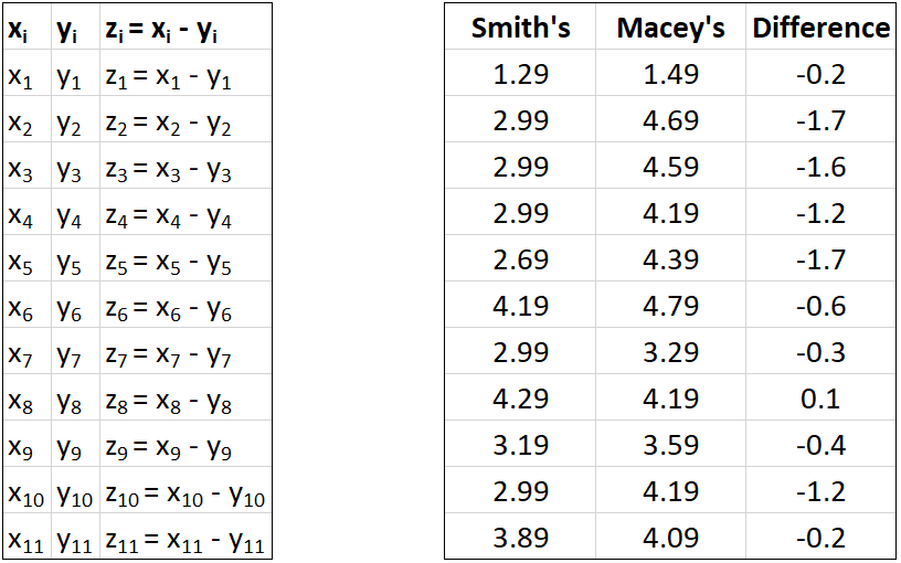
An estimate of $\mu_z$ is the mean of the sample differences: $\bar{z} = \frac{1}{n}\sum_{i=1}^n z_i$. $s.e.(\bar{Z})=s_{\bar{Z}}=\frac{s_z}{\sqrt{n}}$ where $s_z$ is the standard deviation of the differences, $s_z = \sqrt{\frac{1}{n-1}\sum_{i=1}^n(z_i-\bar{z})^2} $
$\bar{z} = \frac{1}{n}\sum_{i=1}^n z_i$
$s.e.(\bar{Z})=s_{\bar{Z}}=\frac{s_z}{\sqrt{n}}$
Step 3: Construct a Test-Statistic
The test statistic for a hypothesis test for the mean difference of paired samples has the same form as the test statistic for the one sample test: $ \texttt{test statistic}=\frac{\texttt{estimate} - \texttt{null value}}{\texttt{s.e.(estimate)}} $. Specifically, $T = \frac{\bar{z}-\delta}{s_z/\sqrt{n}}$. This statistic has a t-distribution with n-1 degrees fo freedom.
$T = \frac{\bar{z}-\delta}{s_z/\sqrt{n}} \sim t_{n-1}$
For the test to determine whether there is a difference in mean prices at the two grocery stores, the test statistic is $T = \frac{-0.818-0}{0.675/\sqrt{11}} = -4.019$.
Step 4: Compute a p-value
The p-value for this test comes from a t-distribution. Whether the p-value comes from one or two tails depends on the form of the alternative hypothesis.
For the test to determine whether there is a difference in mean prices at the two grocery stores, the p-value is 0.002.
Since the alternative hypothesis is $H_A:\mu_z\neq0.$ (two-sided), the p-value includes both tails.
As with all hypothesis tests, we should draw conclusions both statistically and contextually.
The p-value for the grocery store price comparison, 0.002, is very small so we reject the null hypothesis. The results are statistcally significant.
We conclude that there is evidence of a difference in the mean prices of cookies and crackers at the two stores.
Caution: Keep in mind that since our random sample came from cookies and crackers only, we can't general to other products at the grocery stores. It is possible that if we compared other types of products, for instance canned goods, that the results would be different.
A Confidence Interval for Paired Samples
A confidence interval for the mean of the differences of paired samples also has the same basic form as the confidence intervals we have seen previously: $$\text{(estimate }\pm\text{ critical value }\times\text{ standard error of the statistic).}$$ In this case, the estimate is the mean of the differences in the sample, $\bar{z}$, the critical value comes from the t-distribution, and the standard error is the sample standard deviation, $s_z$
\(\left(\bar{z} - t_{n-1, \alpha/2}\frac{s_z}{\sqrt{n}}, \bar{z} + t_{n-1, \alpha/2}\frac{s_z}{\sqrt{n}}\right)\)
Find a 90% confidence interval for the mean difference in prices of cookies and crackers at the two grocery stores.
We saw previously that $\bar{z} = -0.818$ and $s_z=0.675$.
The critical value for a 90% confidence interval from a t-distribution with 10 degrees of freedom is 1.812.
Thus the confidence interval is: $$(-0.818 - 1.812 \times \frac{0.675}{\sqrt{11}}, -0.818 + 1.812 \times \frac{0.675}{\sqrt{11}})$$ $$ = (-1.187, -0.449)$$ Notice that 0 is not in the interval. This agrees with the hypothesis test in indicating that there is evidence that the mean difference is not 0.
Moreover, the values in the interval are all negative and the Macey's prices were subtracted from the Smith's prices, the Macey's cookies and crackers are, on average, more expensive.
Independent Samples
Independent samples arise when measures are made on two unrelated or independent subjects.
Is the mean IMDb rating of Hulu's movies different from the mean rating of movies available on Disney+?
To address this question, it does not make sense to use paired samples. If we chose the same movies from each streaming service, the mean ratings of those movies would, of course, be the same. Instead, we will choose a random sample from each service to be representative of the movies available on that site.
Since this is a question about two populations (Hulu's movies and Disney+ movies) this is still a two sample problem. However, since we choose a random sample from each population, the samples are independent.
The hypothesis testing procedure presented here is called the general procedure and can always be used to compare two independent means. After describing this method and working through an example, we will introduce the pooled-variance procedure, a slightly different process that is more powerful in the case when the underlying population variances are assumed to be equal.
The General Procedure for Comparing Two Means
Step 1: State HypothesesWhen comparing independent samples, the parameter of interest is the difference between the population means: $\mu_A-\mu_B$ where A and B denote the first and second populations respectively. The null hypothesis for a test of independence is: $$H_0: \mu_A-\mu_B = \delta$$ where $\delta$ is again used to denote the null value. The alternative hypothesis will have one of the following forms:
- $H_A: \mu_A-\mu_B \neq \delta$
- $H_A: \mu_A-\mu_B > \delta$
- $H_A: \mu_A-\mu_B < \delta$
Let $\mu_A$ denote the mean IMDb rating of movies available on Hulu and let $\mu_B$ denote the mean IMDb rating of movies available on Disney+. The null and alternative hypotheses for this test are: $$H_0: \mu_A-\mu_B = 0$$ $$H_A: \mu_A-\mu_B \neq 0 $$
Step 2: Collect Data
Collect data by choosing a random sample from each of the two populations to be compared. Consider
- A sample of $m$ observations \(X_1, X_2, \ldots, X_m\) from population $A$, with mean $\bar{X}$ and sample standard deviation $S_x$.
- A sample of $n$ observations \(Y_1, Y_2, \ldots, Y_n\) from population $B$ with mean $\bar{Y}$ and standard deviation $S_y$.
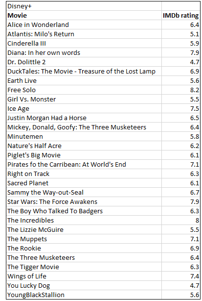
To obtain data to address this question, we used the website reelgood.com the lists all the movies available to stream from a number of streaming services. We obtained data for a random sample of 29 of the movies available from Hulu on June 6, 2020 and a random sample of 30 movies available from Disney+ on the same date. Click on the buttons to see the data.
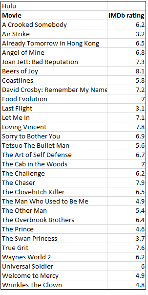
| Hulu IMDb: | $\bar{x} = 6.117$ | $s_x = 1.342$ | $m=29$ |
| Disney+ IMDB: | $\bar{y} = 6.433$ | $s_y = 0.934$ | $n=30$ |
Notice that mean of the Disney+ sample is somewhat larger than that of the Hulu sample. The purpose of the hypothesis test is to determine if this difference is big enough to provide evidence that the population means are also different.
Step 3: Construct a Test-Statistic
The statistic used to estimate the difference in means, $\mu_A-\mu_B$ is $\bar{X}-\bar{Y}$.
For a test of $H_0: \mu_A-\mu_B = \delta$, the test statistic is: $T=\frac{\bar{X} - \bar{Y} - \delta}{\sqrt{\frac{s^2_x}{m} + \frac{s^2_y}{n}}}$. This statistic has an approximate $t_\nu$ distribution. The degrees of freedom, $\nu$ can be estimated using the results of this formula: $$\nu = \frac{\left(\frac{s_x^2}{m}+\frac{s_y^2}{n}\right)^2}{\frac{(s_x^2/m)^2}{m-1}+\frac{(s_y^2/n)^2}{n-1}}$$ The applet below can be used to compute the degrees of freedom.
Test Statistic for a Difference in Two Means, Independent Samples
$T=\frac{\bar{X} - \bar{Y} - \delta}{\sqrt{\frac{s^2_x}{m} + \frac{s^2_y}{n}}}\sim t_{\nu}$
| Hulu IMDb: | $\bar{x} = 6.117$ | $s_x = 1.342$ | $m=29$ |
| Disney+ IMDB: | $\bar{y} = 6.433$ | $s_y = 0.934$ | $n=30$ |
$$T=\frac{6.117 - 6.433 - 0}{\sqrt{\frac{1.342^2}{29} + \frac{0.934^2}{30}}} = -1.046$$ The degrees of freedom are $$\nu = \frac{\left(\frac{1.342^2}{29}+\frac{0.934^2}{30}\right)^2}{\frac{(1.342^2/29)^2}{28}+\frac{(0.934^2/30)^2}{29}} = 49.815$$ Use the applet to verify this result.
Step 4: Compute a p-value
The test statistic has a t-distribution, thus we will use this distributio to compute a p-value. Whether the p-value is obtained from one or two tails depends on the form of the alternative hypothesis.
$$T=-1.046$$ There are 49.815 degrees of freedom.
p-value = $2\times P(t \lt -1.046) = 2 \times 0.150 = 0.3.$
As with all hypothesis tests, we should draw conclusions both statistically and contextually.
The p-value, 0.3, is larger than the significance level of 0.05. Thus we fail to reject the null hypothesis.
There is no evidence that the mean IMDb ratings of the movies available on Hulu and Disney+ differ.
A Confidence Interval for Two Means, Independent Samples
A confidence interval for the mean of the differences of independent samples also has the same basic form as the confidence intervals we have seen previously: $$\text{(estimate }\pm\text{ critical value }\times\text{ standard error of the statistic).}$$ In this case, the estimate is the mean of the differences in the sample, $\bar{x}-\bar{y}$, the critical value comes from the t-distribution, and the standard error is $\sqrt{\frac{s^2_x}{m} + \frac{s^2_y}{n}}$
\(\left(\bar{x}-\bar{y} - t_{\nu, \alpha/2}\sqrt{\frac{s^2_x}{m} + \frac{s^2_y}{n}}, \bar{x}-\bar{y} + t_{\nu, \alpha/2}\sqrt{\frac{s^2_x}{m} + \frac{s^2_y}{n}}\right)\)
$\bar{x}-\bar{y} = -0.316$
$\sqrt{\frac{s^2_x}{m} + \frac{s^2_y}{n}} = 0.302$
$t_{.025,49.815} = 2.009$
95% CI for the difference in means: $$(-0.316 - 2.009(0.302), -0.316 + 2.009(0.302))$$ $$ = (-0.923, 0.291)$$
The Pooled-Variance Procedure for Comparing Two Means
When it can be assumed that the population variances are (approximately) equal, the pooled-variance procedure is more powerful than the general procedure . To determine whether this procedure should be used in preference to the general procedure, since the actual population variances are unknown, compare the sample variances. Use the pooled-variance procedure if the larger sample variance is no more than one and a half times the smaller sample variance.
Use the pooled-variance procedure when the larger sample variance is less than 1.5 times the smaller sample variance.
| Hulu IMDb: | $\bar{x} = 6.117$ | $s_x = 1.342$ | $m=29$ |
| Disney+ IMDB: | $\bar{y} = 6.433$ | $s_y = 0.934$ | $n=30$ |
The larger sample variance is $ 1.342^2 $ and the smaller is $0.934^2$. The ratio of the larger variance to the smaller variance is $1.342^2/0.934^2 = 2.064$ Since the larger sample variance is 2.064 times the smaller sample variance, the general procedure was most appropriate for this analysis.
Is the mean IMDb rating of Netflix movies the same and that of Hulu movies?
To address this question, we selected a random sample of movies available on each of the streaming services in June 2020. Again, since we choose a random sample from each population, the samples are independent. We obtained the following summary statistics for these data:
| Netflix IMDb rating: | $\bar{x} = 6.058$ | $s^2_x = 1.728$ | $m=33$ |
| Hulu IMDb rating: | $\bar{y} = 6.117$ | $s^2_y = 1.800$ | $n=29$ |
The ratio of the larger sample variance to the smaller is $1.800/1.728 = 1.04$. Since the sample variances are nearly the same, it is safe to assume that the population variances are also approximately equal. We will conduct a hypothesis test using the pooled-variance procedure.
The overarching hypothesis testing procedure is the same for the general procedure and the pooled-variance procedure. The differences in the details are in computation of the standard error and degrees of freedom.
The Standard Error for the Pooled-Variance Procedure for Two Means
$S_p\sqrt{\frac{1}{m}+\frac{1}{n}}$ where $S_p = \frac{(m-1)S^2_x+(n-1)S^2_y}{m+n-2}$
This test statistic has a t-distribution with $m+n-2$ degrees of freedom.
Degrees of Freedom for the Pooled-Variance Procedure for Two Means
$\nu = m+n-2$
The test statistic is $T = \frac{\bar{X}-\bar{Y} - \delta}{S_p\sqrt{\frac{1}{m}+\frac{1}{n}}}\sim t_{m+n-2}$
- State Hypotheses: Let $\mu_A$ denote the mean IMDb rating of movies available on Netflix and let $\mu_B$ denote the mean IMDb rating of movies available on Hulu. The null and alternative hypotheses for this test are: $$H_0: \mu_A-\mu_B = 0$$ $$H_A: \mu_A-\mu_B \neq 0 $$
- Collect Data: We chose a random sample of 33 movies from the Netflix catalog and a random sample of 29 movies from the Hulu catalog in June 2020
and obtained the following summaries:
Netflix IMDb rating: $\bar{x} = 6.058$ $s^2_x = 1.728$ $m=33$ Hulu IMDb rating: $\bar{y} = 6.117$ $s^2_y = 1.800$ $n=29$ - Construct a test statistic:
$S_p = \frac{(m-1)s^2_x+(n-1)s^2_y}{m+n-2}=\frac{32(1.728)+28(1.800)}{33+29-2} = \frac{105.696}{60} = 1.762$
$T = \frac{\bar{X}-\bar{Y} - \delta}{S_p\sqrt{\frac{1}{m}+\frac{1}{n}}} = \frac{6.058-6.117 - 0}{1.762\sqrt{\frac{1}{33}+\frac{1}{29}}}=-0.132$ - Compute a p-value: $T\sim t_{m+n-2} = t_{60}$
p-value = $2\times P(t_{60} < -0.132) = 0.895$ - Draw Conclusions: The p-value, 0.895, is larger than 0.05. We fail to reject the null hypothesis. There is no evidence that the mean IMDb ratings of the movies available on Netflix and Hulu differ.
A Confidence Interval for Independent Samples, Pooled-Variance Procedure
Again, a confidence interval based on the pooled-variance procedure for two means has the same basic form as the confidence intervals we have seen previously: $$\text{(estimate }\pm\text{ critical value }\times\text{ standard error of the statistic).}$$ In this case, the estimate is the mean of the differences in the sample, $\bar{x}-\bar{y}$, the critical value comes from the $t_{m+n-2}$-distribution, and the standard error is $S_p\sqrt{\frac{1}{m}+\frac{1}{n}}$
\(\left(\bar{x}-\bar{y} - t_{\nu, \alpha/2}\,\,S_p\sqrt{\frac{1}{m}+\frac{1}{n}},\,\, \bar{x}-\bar{y} + t_{\nu, \alpha/2}\,\,S_p\sqrt{\frac{1}{m}+\frac{1}{n}}\right)\)
$\bar{x}-\bar{y} = -0.059$
$S_p\sqrt{\frac{1}{m}+\frac{1}{n}} = 1.762*\sqrt{\frac{1}{33}+\frac{1}{29}} = 0.448$
$t_{.025,60} = 2$
95% CI for the difference in means: $$(-0.059 - 2(0.448), -0.059 + 2(0.448))$$ $$ = (-0.955,0.837 )$$