Probability Models and Random Variables

The Virginia Lottery offers a game called the New Year's Millionaire Raffle for which the top prize is one million dollars. There are 375,000 tickets sold, of which 508 are winners. There are three top prizes of $\small{\$1,000,000}$, five second prizes worth $\small{\$100,000}$, and 500 third prizes worth $\small{\$500}$ each. If we think of buying a raffle ticket as conducting a simple experiment, then the possible outcomes for the experiment could be expressed as winning top prize, a second prize, a third prize, or nothing.

A probability model is a convenient way to describe the distribution of the outcomes of an experiment. It consists of all the possible outcomes of an experiment their corresponding probabilities. It is often useful to display the probability model with a table.

A probability model consists of the experimental outcomes and their probabilities.

A probability model for the Virginia raffle looks like this. Table showing the probabilities for four possible outcomes in a prize drawing. The outcomes are Top Prize, Second Prize, Third Prize, and No Prize. The corresponding probabilities are 3 out of 375,000 for the Top Prize, 5 out of 375,000 for the Second Prize, 500 out of 375,000 for the Third Prize, and 374,492 out of 375,000 for No Prize.

Table showing the probabilities for four possible outcomes in a prize drawing. The outcomes are Top Prize, Second Prize, Third Prize, and No Prize. The corresponding probabilities are 3 out of 375,000 for the Top Prize, 5 out of 375,000 for the Second Prize, 500 out of 375,000 for the Third Prize, and 374,492 out of 375,000 for No Prize.

What is a random variable?

The sample spaces S={top prize, second prize, third prize, no prize} and S={1000000,100000,500,0} refer to the same outcomes in different ways. In the second sample space, prize status is indicated by the amount of money associated with each prize. We could define a variable X such that \[ X = \begin{cases} 1,000,000 & \text{if top prize} \\ 100,000 & \text{if second prize} \\ 500 & \text{if third prize}\\ 0 & \text{if no prize}\\ \end{cases} \] A variable that assigns each outcome in a sample space to a real number is called a random variable. Random variables enable us to work mathematically with experimental outcomes. For instace, for the VA lottery, we can use random variables to describe how much money lottery players will win on average, how much the winning will vary, or and how much someone who bought multiple tickets would win, on average.

$\rightarrow$ A random variable maps each outcome of an experiment to a real number.

NOTATION
A random variable is usually denoted with a capital letter from near the end of the alphabet. X, Y, and Z are common.

Observed values of a random variable are denoted by corresponding lower-case letters, thus x or x₁,x₂...x_n denote the specific values that the random variable X can take on.

The notation P(X = x) means 'the probability that random variable X assumes value x'.

Discrete and Continuous Random Variables

Random variables can be discrete or continuous.

The outcomes of a discrete random variable are countable. That means they can be mapped to the integers or a subset of the integers. E.g. the number of students in a randomly selected class or the number of times someone rolls two dice before they get doubles. Notice that countable is not the same as finite. For instance, the number of times a student sneezes in a hour is countable but has no definite upper limit.

A continuous random variable is defined over an interval or intervals and is, therefore, always infinite. The time it takes to fill a randomly selected car with gas and the length of time between spotting shooting stars are continuous random variables.

$\rightarrow$ A discrete random variable has countable outcomes.

$\rightarrow$ A continous is defined over an interval or intervals.

Example: Which of the following describe discrete random variables? Which describe continuous random variables?
W: The outcome of a die roll.
X: The number of 6's in 10 die rolls.
Y: The weight of a randomly chosen die.
Z: The length of time a rolled die tumbles.

W and X are discrete random variables. Y and Z are continuous.

W and Y are discrete random variables. X and Z are continuous.

The Distribution of a Random Variable

Much of statistics and probability is concerned with describing the distributions of random variables, that is the values that the variable can assume and the probabilities of those outcomes. For instance, consider the variable: the outcome of a die roll. The distribution of this variable would indicate that the possible values are the numbers 1, 2, 3, 4, 5, 6 and that these outcomes are all equally likely, each with probability 1/6. This information can be presented in a graph, table, or formula.

$\rightarrow$ The distribution of a random variable describes the possible outcomes and their associated probabilities.

In the case of a discrete random variable, such as the outcome of a die roll, a table displays the distribution by listing the possible outcomes with their probabilities. A graph shows bars at each of the possible outcomes with height corresponding to the probability of that outcome.

A probability distribution graph showing six vertical orange bars of equal height at positions 1 through 6, each with a probability of 1/6. The x-axis ranges from 0 to 7, representing possible outcomes of rolling a fair six-sided die.

A table showing the probability distribution for rolling a fair six-sided die. The top row lists outcomes 1 through 6, and the bottom row lists the probability for each outcome as 1/6.

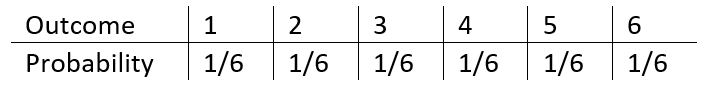
The table and the graph both show the distribution of the outcome of a die roll.

Since there are infinite possible outcomes for a continuous random variable, the distribution cannot be displayed in a table, rather it is described with a formula or graph.

Example: A machine that fills 15oz chip bags has been calibrated to slightly overfill. The distribution of the weight, W, of the chips in the bag might be described by a formula such as $\small{f(w) = 8.5-\frac{x}{2}}$ for $\small{15 \leq w \leq 17}$. The graph of this distribution is shown.

A simple line graph with orange segments connecting data points. The x-axis ranges from 14 to 18. The line remains flat from 14 to 15, rises steeply between 15 and 16, then slopes downward to reach zero at 17, and stays flat through 18.

For every distribution, the probabilities are all non-negative and the total probabilty is 1.