Amusement park patrons, wanting to go on a log ride, might not have to wait in line at all, they might have to wait for
hours, or the wait could be anywhere in between. For a random log rider, the wait time can be indicated by a continuous random variable.
A continuous random variable maps the outcomes of a chance process to an interval or intervals.
It has an infinite number of possible outcomes. Variables corresponding to outcomes that are are measured are continuous.
Suppose the wait time for the log ride at
an amusement park is 2 hours or less. Let W be a random variable that indicates the wait time of a randomly chosen customer.
W can assume any value between 0 and 2. The wait could be 0.5 hours or 0.6 hours or 0.55 hours, etc. - there are infinite possibilities.
W is a continuous random variable.
The Distribution of a Continuous Random Variable
Graphs and formulas describe the distribution of a continuous random variable. These indicate the observable values
of the random variable and associated probabilities. As with discrete random variables, it is sometimes convenient to work with probabilities directly
and sometimes to work with cumulative probabilities.
The formulas and graphs below all describe the same possible distribution of W, the wait time for the log ride of a randomly chosen amusement park visitor.
Two ways of describing one possible distribution
of W are shown here in both formula and graphical forms.
Probability Density Function
Cumulative Distribution Function
Formula
$\small{f(x) = 1-\frac{x}{2}, \text{ for } 0\leq x \leq 2}$
$\small{F(x) = x-\frac{x^2}{2/4}, \text{ for } 0\leq x \leq 2}$
Graph
The Probability Density Function
The probability density function (pdf) describes the distribution of a continuous random variable. The probability that
a random variable assumes an outcome in a given interval are computed by finding the area under the function over that interval. The pdf is usually
indicated in function notation.
→ A probability density function (pdf) is a function that describes the
distribution of a continuous random variable.
For a continuous random variable $X$ that can take values between $l$ and $u$, we denote
the pdf of $X$ by $f(x)$, for $l \leq x \leq u$. The interval from $l$ to $u$ is called the
support of the random variable, or the set of values where the probability is non-zero.
If no specific interval is indicated, it is assumed that the support is all
real numbers.
NOTATION: The probability density function is denoted 'f(x), l ≤ x ≤ u'.
→ The support of a random variable consists of the interval or intervals where the density function is non-zero.
Suppose the distribution of W, the wait time for the log ride of a randomly chosen park visitor, is described by the probability density function
$\small{f(x) = 1-\frac{x}{2}, \text{ for } 0\leq x \leq 2}$
From the graph, we can see that while all the wait times are between 0 and 2 hours,
shorter wait times are more likely.
Notice that the pdf is 0 except between 0 and 2. That means that no wait will
be less than 0 hours and none will be longer than 2 hours.
A pdf satisfies these properties:
$f(x) \geq 0$ for all $x$ (all probabilities are greater than or equal
to 0)
$\int_l^u f(x)dx = 1 $ (the probability that the the random variable takes on a value between $l$ and $u$ is 1.)
Suppose, W, the wait time for the log ride of a randomly chosen park visitor has the probability density function
$\small{f(w) = 1-\frac{w}{2}, \text{ for } 0\leq w \leq 2}$
Show that $f$ satisfies the above properties.
$f(w) \geq 0$: The graph shows that the function is non-negative on the
interval $0 \leq w \leq 2$.
To participate in a wrestling tournament, high school wrestlers must measure below a specified weight for their weight class. Let X denote the difference
between a randomly chosen wrestler's weight and the indicated weight for their class. If $f(x) = -A(x^2+2x-3) \text{ for } -2\leq x \leq 1$, what
is the value of $A$ that makes this a pdf?
If $f(x)$ is a pdf then $\int_{-2}^1-A(x^2+2x-3d)x = 1$.
$\int_{-2}^1-A(x^2+2x-3)dx = 9A = 1$ so $A=\frac{1}{9}$.
Finding Probabilities with the Probability Density Function
The probability that a continuous random variable takes on a value in a given interval is equal to the area under the pdf
over that interval. Thus, to find the probability that a continuous random variable takes on a value over a given interval, integrate over that interval.
$P(a\leq x \leq b)$ indicates
The probability that an individual randomly selected from the underlying
population will have a value of X that falls between a and b.
The proportion of individuals in the underlying population that have a value
of X between a and b.
Use the applet to explore finding a probability with a pdf.
Drag the points labelled 'a' and 'b' to change the interval of interest.
'b' will adjust with 'a' so move 'a' first.
What happens when a < 0 or b > 2?
Find the probability that the waiting time for an amusement park visitor to ride the log ride is between 1 and 1.5 hours.
The probability density function for wait time is
$\small{f(w) = 1-\frac{w}{2}, \text{ for } 0\leq w \leq 2}$
The probability that someone waits between 1 and 1.5 hours for the log ride is 0.1875.
Use the applet to verify this answer!
To participate in a wrestling tournament, high school wrestlers must measure below a specified weight for their weight class. Let X denote the difference
between a randomly chosen wrestler's weight and the indicated weight for their class. $f(x) = -\frac{1}{9}(x^2+2x-3) \text{ for } -2\leq x \leq 1$. What is
the probability that a wrestler exceeds the stated weight?
A wrestler exceeds the given weight if the difference between their weight and that indicated weight is greater than 0.
The probability that a wrestler is over the weight is 0.19, that is, about 19% of wrestlers are over the weight.
To find the probability that a mature tree is taller than 150 feet, or that X
is greater than 1.5, we integrate from 1.5 to 3 (the pdf is in terms of hundreds
of feet).
If X is a continuous random variable then $P(X=x) = 0$.
The probability that a continuous random variable takes on a value in an
interval, $(a,b)$, is the area under the density function between $a$ and $b$ and is found with integration, $P(a \leq X \leq b) = \int_a^b f(x)dx$.
For a single value, $a$, $P(X = a) = \int_a^a f(x)dx = 0$.
Another way to think of this is that for a continuous random variable, there are infinite
possible values so the probability that X takes on a specfic value is 0, i.e. $P(X=a) = \frac{1}{\infty} = 0$. Thus, if X is a continuous random variable,
$P(X \leq a)$ and $P(X \lt a)$ are equivalent.
The Cumulative Distribution Function
To find a probability with a probability density function, integrate over the interval of interest. To find the probability
over a different interval, integrate again.
Like the probability density function, the cumulative distribution function describes the distribution of a random variable,
however, we integrate the pdf to find the cdf, so the integration step is done up front and probabilities can be found simply by plugging values into the
function and evaluating.
→ The cumulative distribution function (cdf) of a continuous random variable $X$ is a function that describes the
distribution of a continuous random variable in terms of cumulative probabilities.
The notation $F(x)$ denotes the cdf of $X$. Using '$F$' for the cdf and '$f$' for
the pdf suggests the relationship between the functions. Just as in calculus, we use
the $'F'$ to denote the antiderivative of $'f'$.
As with the pdf, it is important to always indicate the support when reporting a cdf. If
no support is given, assume that the support is all real numbers.
NOTATION:
Both 'F(x)' and 'P(X ≤ x)' denote the cumulative distribution function of X. F(x) = P(X ≤ x).
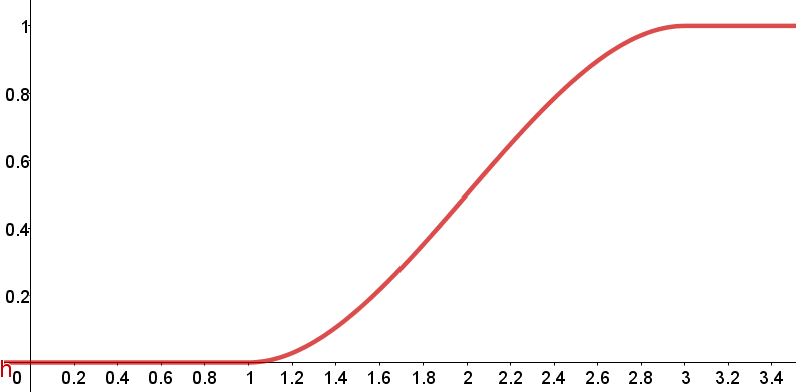
W, the wait time for the log ride of a randomly chosen amusement park visitor has cumulative distribution function
$\small{F(w) = w-\frac{w^2}{4}, \text{ for } 0\leq w \leq 2}$
The height of the graph at point w corresponds to the probability that the wait time is no longer
that w hours.
The cdf is 0 below 0 since no wait time will be less than 0 hours. It is 1 above 2 since 2 hours is the longest
wait time according to this model.
A cdf satisfies these properties:
$F(x) \rightarrow 0$ as $x \rightarrow -\infty$.
$F(x)$ is non-decreasing.
$F(x) \rightarrow 1$ as $x \rightarrow \infty$.
Finding the CDF from the PDF
The cdf of $X$ is the integral of the pdf of $X$. If $X$ has pdf $f(x)$ for $l \leq x \leq u$, $F(y) = P(X \leq y)$. (Use '$y$' here for
convenience). Since $F(y) = 0$ for $y \leq l$, $$\small{\begin{array}{rcl} F(y) & = & P(X \leq y)\\ & = & P(l \leq x \leq y)\\ & = & \int_l^yf(x)dx\end{array}}$$
Suppose, W, the wait time for the log ride of a randomly chosen park visitor has the probability density function
$\small{f(w) = 1-\frac{w}{2}, \text{ for } 0\leq w \leq 2}$. Find the cdf of w.
Changing the variable back to w, $\small{F(w) = w - \frac{w^2}{4} \text{ for } 0 \leq w \leq 2}$.
Finding Probabilities with the CDF
Whereas to find $P(X\leq x)$ using the probability density function, it is necessary to integrate, finding $P(X\leq x)$
using the cumulative distribution function, entails plugging in a value for x and evaluating.
W, the wait time for the log ride of a randomly chosen park visitor has the probability density function
$\small{f(w) = 1-\frac{w}{2}, \text{ for } 0\leq w \leq 2}$ and cumulative distribution function
$\small{F(w) = w - \frac{w^2}{4} \text{ for } 0 \leq w \leq 2}$. Find the probability that the wait is less than 45 minutes (0.75 hours)
using the pdf, then find it again using the cdf.
Using the pdf, $\small{f(w) = 1-\frac{w}{2}, \text{ for } 0\leq w \leq 2}$
Use the applet to explore finding a probability with a cdf.
Drag the point $w$ to use the applet to find $P(W \leq w)$.
Investigate what happens if w is less than 0 or greater than 2.
The cdf can also be used to find the probability that a random variable,
$X$, takes on a value over an interval $(a, b)$, $P(a \leq X \leq b) = F(b)-F(a)$.
$P(X \leq a) = F(a)$
$P(a \leq X \leq b) = F(b)-F(a)$
$P(X > a) = 1-F(a)$
Use applet to find the $P(a \leq X \leq b)$ via the pdf or the cdf.
Drag the endpoints of the interval in either graph.
The endpoints in both graphs will change together.
To participate in a wrestling tournament, high school wrestlers must measure below a specified weight for their weight class. Let X denote the difference
between a randomly chosen wrestler's weight and the indicated weight for their class. $f(x) = -\frac{1}{9}(x^2+2x-3) \text{ for } -2\leq x \leq 1$.
Find the cdf of X.
Use the cdf to find the probability that a wrestler's weight is within one half pound of the specified weight.
The probability that a wrestler is over the weight is 0.19, that is, about 19% of wrestlers are over the weight.
To find the cdf of $X$, integrate $f(x)$ from 1 to $y$:
$\small{\int_1^y -0.75x^2+3x-2.25dx = -0.25y^3+1.5y^2-2.25y+1}$, so
$\small{F(x) = -0.25x^3+1.5x^2-2.25x+1, 1 \leq x \leq 3}$.
A percentile is a value $T_p$ such that the random variable, $X$, takes on a value less
than $T_p$ $p\%$ of the time, that is, $F(T_p) = \frac{p}{100}$. Divide $p$ by 100 to express
the result as a probability rather than a percentage.
To find the pth percentile, solve the equation $F(T_p) = \frac{p}{100}$.
The pth percentile of the distribution of a random variable is the value, $T_p$ such that $P(X\leq T_p) = \frac{p}{100}$
W, the wait time for the log ride of a randomly chosen park visitor has cumulative distribution function
$\small{F(w) = w - \frac{w^2}{4} \text{ for } 0 \leq w \leq 2}$. Find and interpret the 30th percentile.
Let $T_{30}$ denote the 30th percentile then $F(T_{30}) = 0.3$. To simplify notation, use T in place of $T_{30}$ in the computations.
Solving this, gives three possible solutions: 0.148, 2.274, and 3.579.
Only one of those, 2.274,
is within the support of $1 \leq X \leq 3$, so $T_{70} = 2.274$.
70% of the trees in the Redwood forest have a height of 227.4 feet or less.