Stat5810
Jingjing Wang
Homework10
1.Rweb
Problem 1:
Recall the exercise we tried in class in Lecture 10 (05/23). We used the student data available on
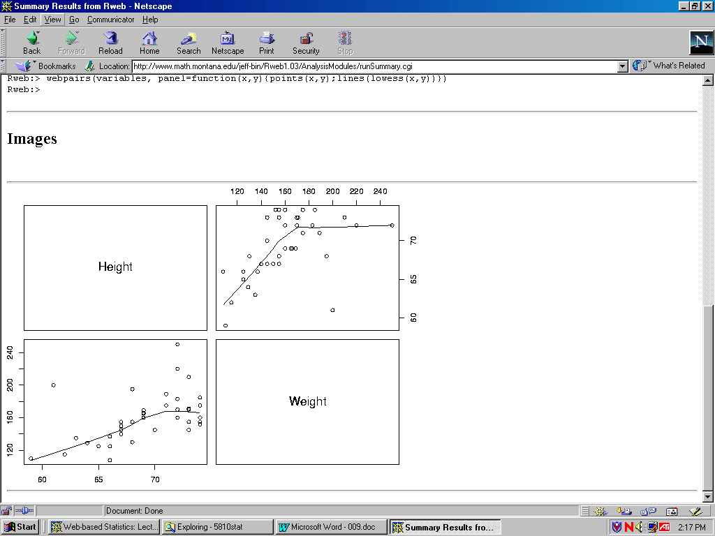
http://www.math.usu.edu/~vukasino/teaching/spring2000/complab/student_data1.prn and used the JavaScript version of Rweb to obtained summary statistics for the variables Age and Siblings. Now try yourself to calculate a few more summary statistics such as the median and the variance of Height and Weight. First make sure to identify the appropriate columns of the matrix X that represent these two variables. Can you also calculate the correlation between these two variables and draw a scatterplot of Height (horizontal) vs. Weight (vertical)?Solution:
Summary ResultsHeight Weight Min. : 59.00 Min. : 108.0 1st Qu.: 67.00 1st Qu.: 142.5 Median : 69.00 Median : 155.0 Mean : 69.12 Mean : 159.9 3rd Qu.: 72.50 3rd Qu.: 173.0 Max. : 74.00 Max. : 250.0 Std Dev: 3.98 Std Dev: 28.9 Rweb:> cor(variables) Height Weight Height 1.0000000 0.5379353 Weight 0.5379353 1.0000000 Rweb:> webpairs(variables) Rweb:>
Images: the graphic on the lower left corner is the scatterplot of Height vs. Weight.
Problem 2:
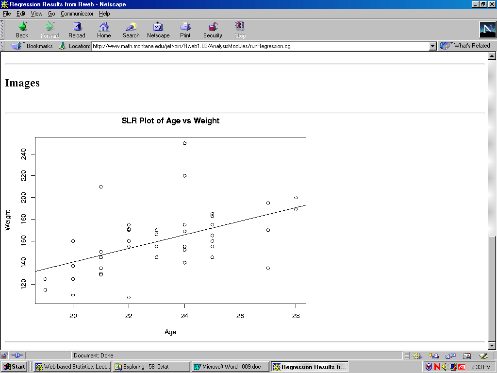
Also, recall how we calculated simple linear regression of Siblings on Age. Now try yourself to calculate a simple linear regression where Weight is the response and Age is the predictor variable. The required syntax is result <- lm(response ~ predictor). Here, result <- means that we assign the outcome of the calculation right of <- to a new variable called result. lm represents a function that calculates a linear model. response ~ predictor represents the expression that should be calculated. You have to replace response and predictor with the appropriate columns of the matrix X. Finally, you have to produce some visible output using the command summary (result).
Solution:
Regression Results:
You are using Rweb1.03 on the server at www.math.montana.edu
Response: Weight
Predictors: Age
R : Copyright 2000, The R Development Core Team
Version 0.99.0 Patched (February 9, 2000)
R is free software and comes with ABSOLUTELY NO WARRANTY.
You are welcome to redistribute it under certain conditions.
Type "?license" or "?licence" for distribution details.
R is a collaborative project with many contributors.
Type "?contributors" for a list.
Type "demo()" for some demos, "help()" for on-line help, or
"help.start()" for a HTML browser interface to help.
Type "q()" to quit R.
Rweb:> postscript(file= "/tmp/Rout.3032.ps", height = 6, width = 8)
Rweb:> X <- read.table("/tmp/Rdata.3032.data", header=T)
Rweb:> attach(X)
Rweb:> names(X)
[1] "Nr." "Gender" "Age" "Siblings" "Eyecolor" "Major" "Height"
[8] "Weight"
Rweb:>
Rweb:>
Rweb:> str <- lm(Weight ~ Age )
Rweb:> residuals <- residuals(str)
Rweb:> predicted <- fitted.values(str)
Rweb:> summary(str)
Call:
lm(formula = Weight ~ Age)
Residuals:
Min 1Q Median 3Q Max
-49.500 -14.462 -1.769 9.904 84.308
Coefficients:
Estimate Std. Error t value Pr(>|t|)
(Intercept) 15.231 38.134 0.399 0.691668
Age 6.269 1.645 3.812 0.000455
Residual standard error: 25.09 on 41 degrees of freedom
Multiple R-Squared: 0.2617, Adjusted R-squared: 0.2437
F-statistic: 14.53 on 1 and 41 degrees of freedom, p-value: 0.0004551
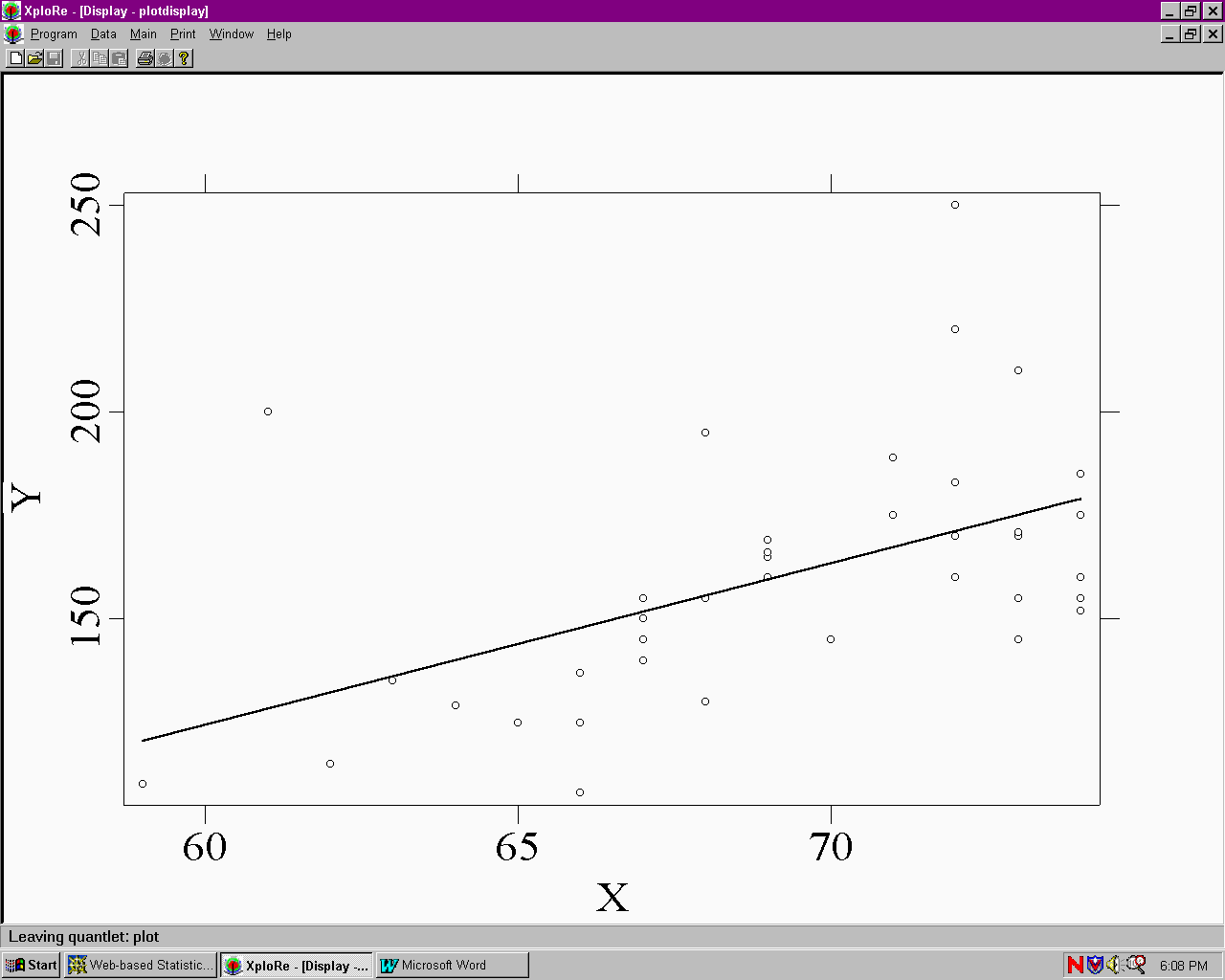
Rweb:> plot(Age, Weight, main="SLR Plot of Age Vs Weight")
Rweb:> abline(lm(Weight ~ Age))
Rweb:>
Images
2.Rice Virtual Lab in Statistics - Data Analysis
Homework problems
Using Rice's Data Analysis Lab Package, solve the problems listed below. Describe exactly all steps needed to obtain the required results (including data editing/recoding). If you encounter any problem (e.g., if a certain applet is not working or if you can clearly see that the results are wrong) mention this explicitly in your written report.
1) Obtain summary statistics for "Height" and "Weight". Also obtain possible graphical displays for these variables.
Solution:
1. Enter http://www.ruf.rice.edu/~lane/rvls.html homepage ,
2. Click on "Analysis Lab" to activate the program
3. When the page is fully loaded, click on the "Analyze" button
4. By clicking on Enter/Edit User Data a clipboard will appear
5. Now open the following file:
http://www.math.usu.edu/~vukasino/teaching/spring2000/complab/student_data1.prn.
6. However, we cannot use this data directly, because it contains non- numerical values. The Data Analysis Lab requires all data to be numeric. So first we have to recode the nonnumeric variables (Gender, Eyecolor, Major) and replace them by the coding integer values, ranging from 1 to the number of levels of the variable. To recode the data, open the file in a text editor that has a "Replace" function (such as Word, Wordpad, UNIX Textedit) and recode the non-numerical variables as follows:
7. After recoding the data, while still in the text editor, select "Select all" from the "Edit" menu and then "Copy". Then change to the Data Analysis Clipboard window and paste the data (by clicking on "Paste" in the "Data" menu at the top of the window).
8. Click on Accept Data. The clipboard window disappear.
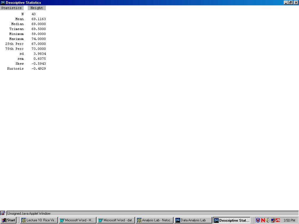
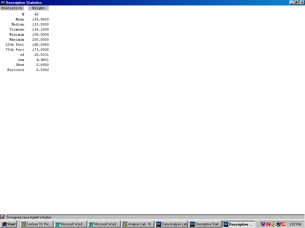
9. When the data are accepted, the names of the variables will appear in the window on the right. In the selection menu on the left, choose Height as dependent . Click Descriptive and got the following Summary statistics for Height:
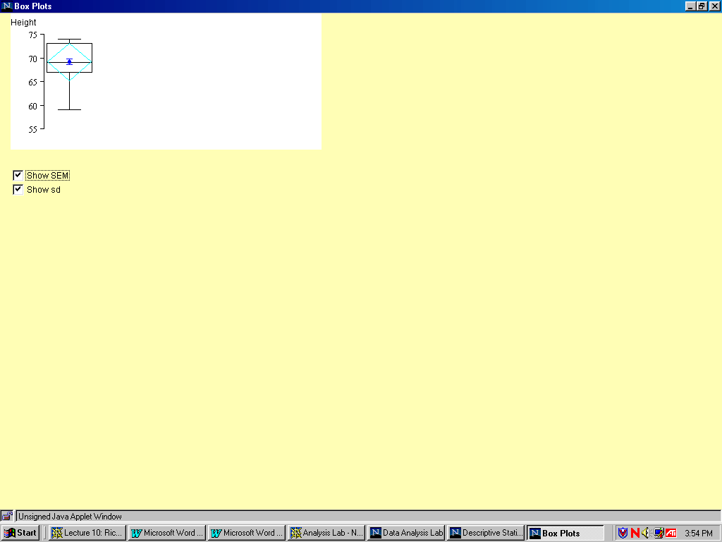
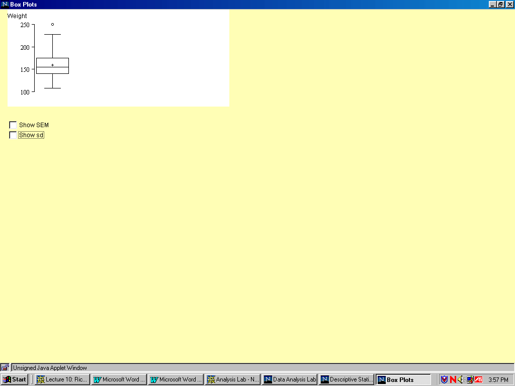
10. Click and got Boxplot for Height:
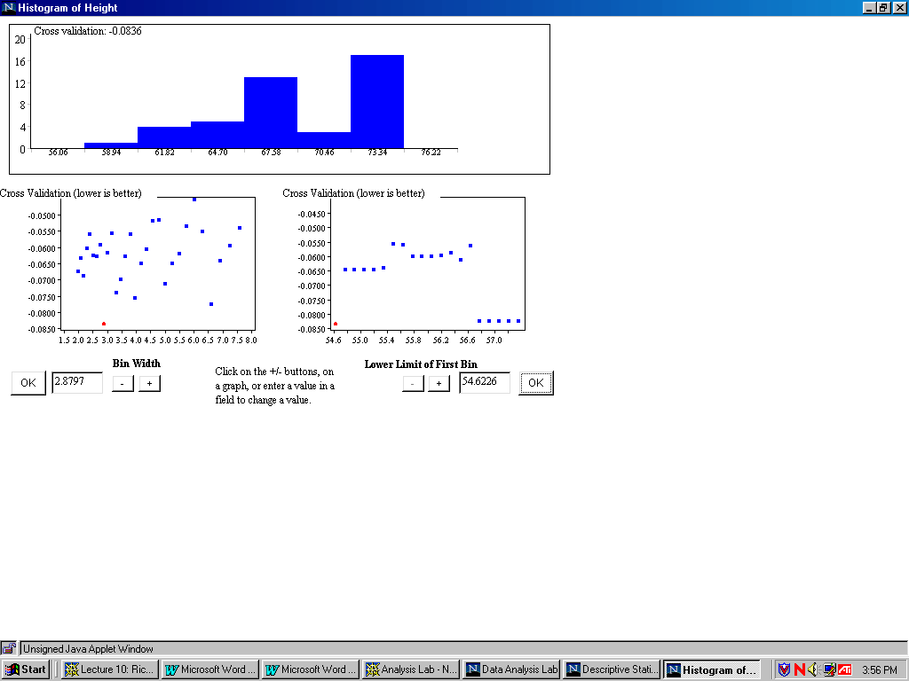
11. Click Histogram and got the Histogram plot for Height:
12. Then go back to the Analysis Lab and choose Weight as dependent. Click Descriptive, and got Summary statistics for Weight:
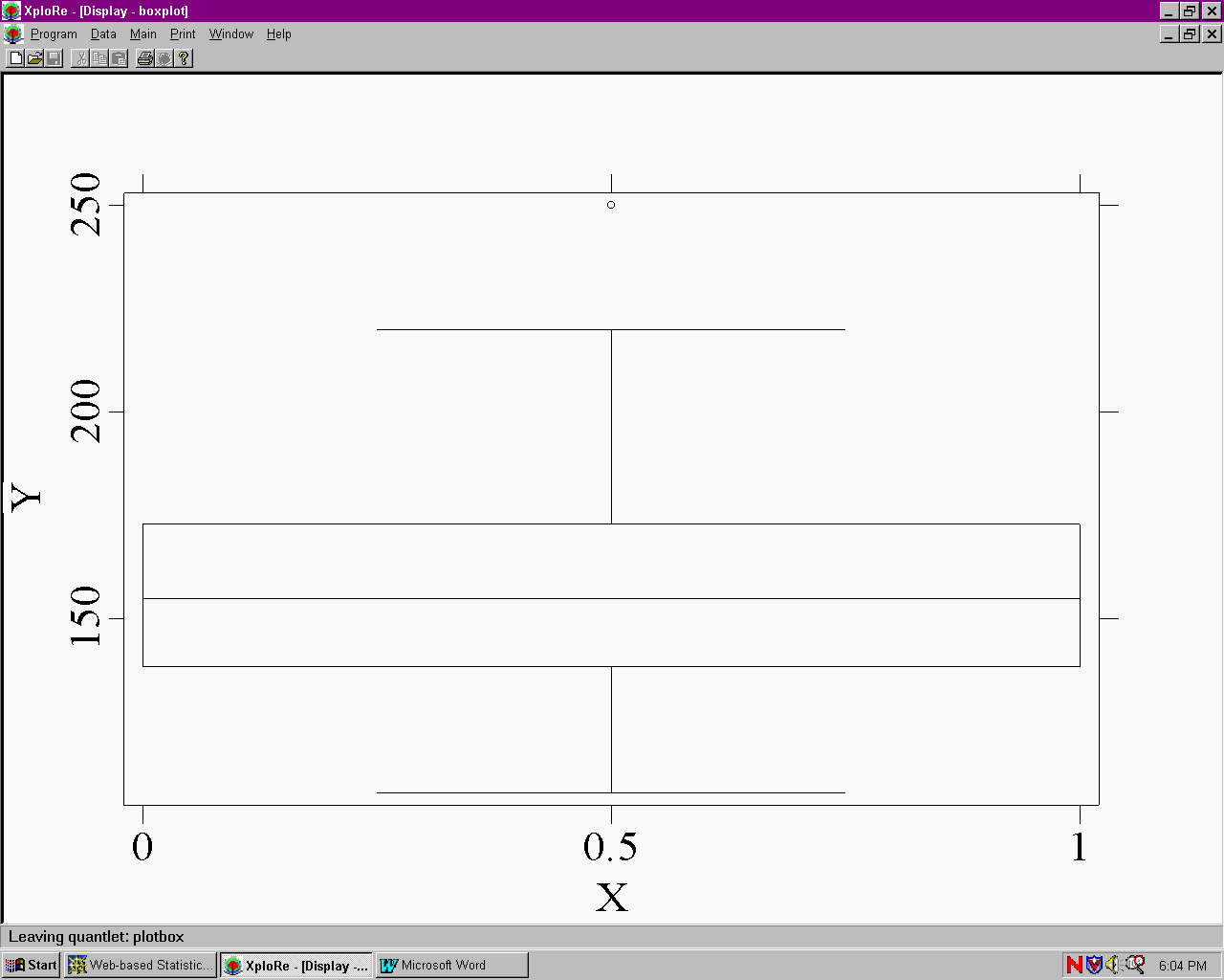
13. Click Boxplot and got Boxplot for weight:
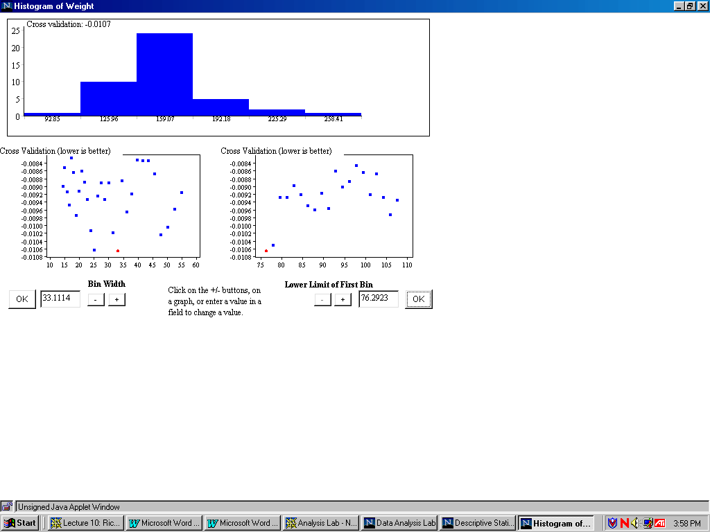
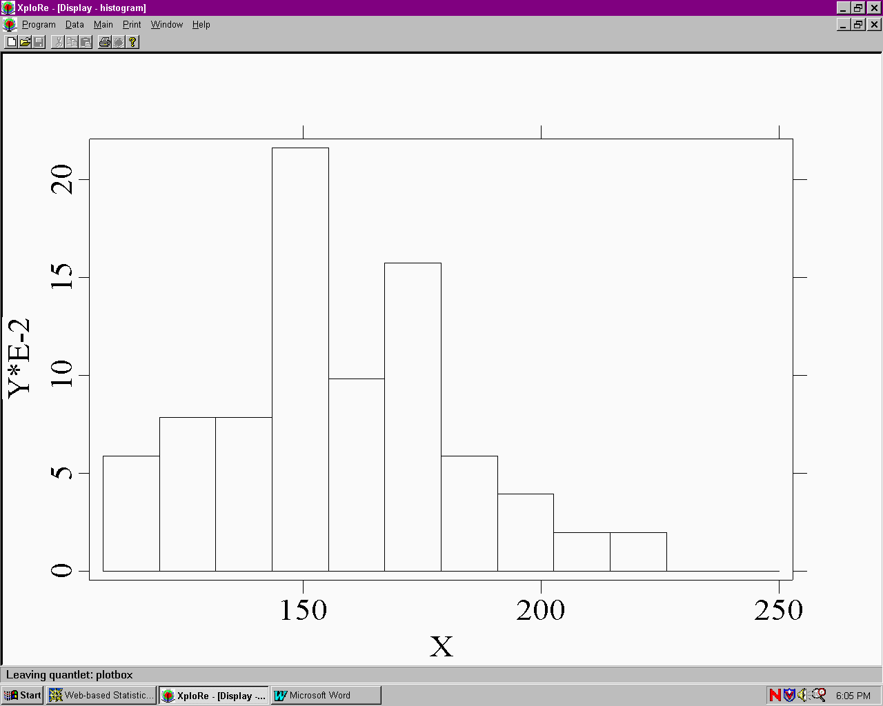
14. Click Histogram and got Histogram for weight:
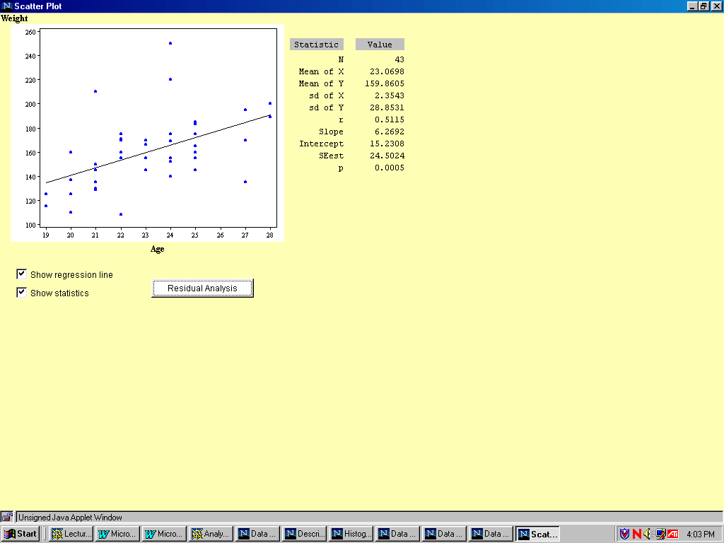
2) Perform a regression analysis of weight on age. What is the predictor variable? What is the dependent variable?
Solution:
1. Choose age as predictor variable and weight as dependent variable.
2.Click Correlation/Regression and got the result as following:
3) Does color of eyes (variable "Eyecolor") have significant influence on weight? Answer this question by carrying out an ANOVA analysis.
Solution:
1.Choose Weight as dependent, Eyecolor as predictor and Eyecolor as grouping variable. Then click ANOVA and get the following analysis:
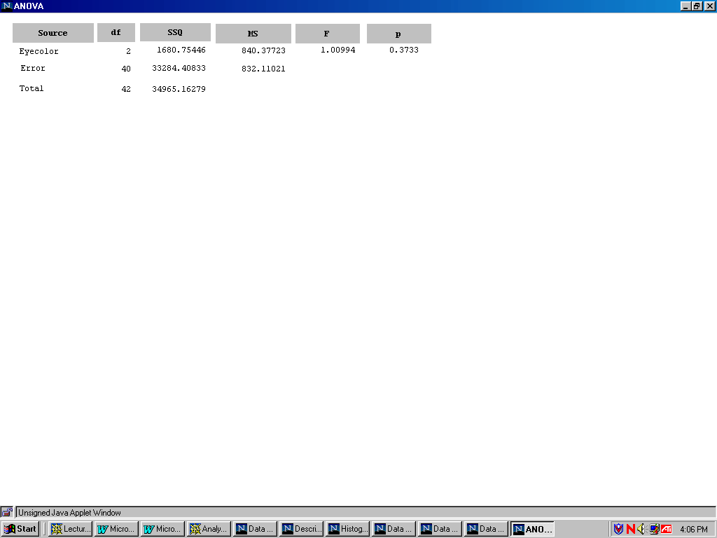
From the above we know that the P value is greater than 0.05, so color of eyes (variable "Eyecolor") have no significant influence on weight.
3. Xplore
Homework:
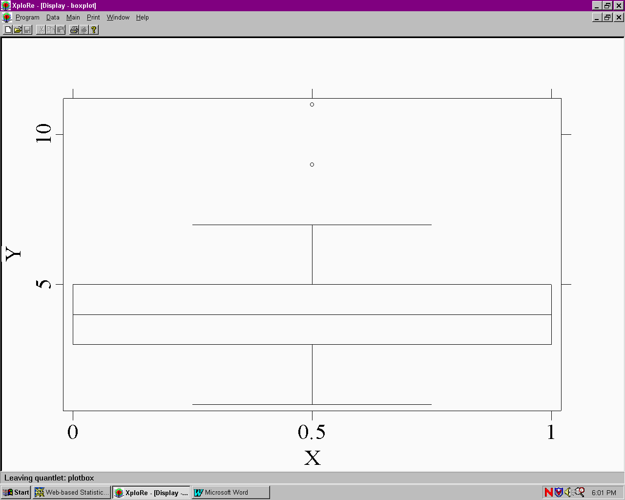
1.Write a program to plot the histogram and boxplot for sibling and weight ,
respectively.
Solution:
1)//Program for histogram & boxplot of Sibling:
library("XploRe")
x = readm("user")
z = x.double[ , 3]
library ("plot")
plothist(z)
plotbox(z)
Boxplot of sibling:
Histogram of Sibling:
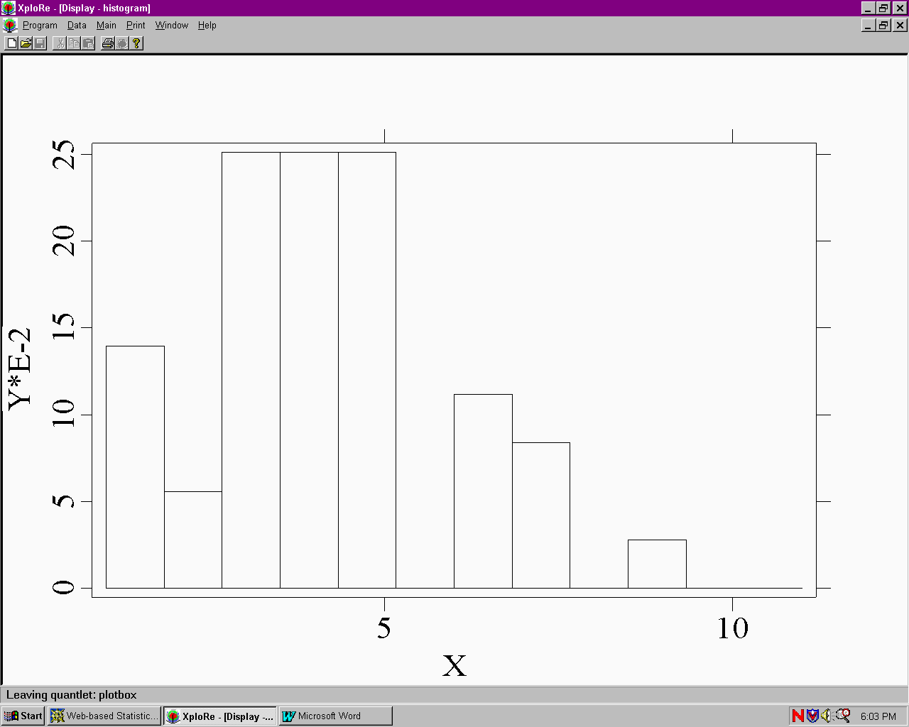
2) //program for histogram & boxplot of weight
library("XploRe")
x = readm("user")
z = x.double[ , 5]
library ("plot")
plothist(z)
plotbox(z)
Boxplot for Weight:
Histogram for Weight:
2.Write a program to perform the regression analysis and plot the regression line of Weight on height.
//program for regression analysis
library("XploRe")
x = readm("user")
y = x.double[ , 4|5]
y1 = y[ , 1]
y2 = y[ , 2]
library("stats")
{b, bse, bstan, bpval} = linreg(y1, y2)
library("plot")
plot(y)
regy=grlinreg(y)
plot(y, regy)
The regression line of Weight on height :
Output of ANOVA:
Contents of string[1,] "readm: Found   43 line(s) and    8 column(s)"

Contents of out[ 1,] ""
[ 2,] "A  N  O  V  A                   SS      df     MSS       F-test   P-value"
[ 3,] "_________________________________________________________________________"
[ 4,] "Regression                 10118.023     1 10118.023      16.696   0.0002"
[ 5,] "Residuals                  24847.140    41   606.028"
[ 6,] "Total Variation            34965.163    42   832.504"
[ 7,] ""
[ 8,] "Multiple R      = 0.53794"
[ 9,] "R^2             = 0.28937"
[10,] "Adjusted R^2    = 0.27204"
[11,] "Standard Error  = 24.61763"
[12,] ""
[13,] ""
[14,] "PARAMETERS         Beta         SE         StandB        t-test   P-value"
[15,] "________________________________________________________________________"
[16,] "b[ 0,]=       -109.4509      66.0171       0.0000        -1.658   0.1049"
[17,] "b[ 1,]=          3.8965       0.9536       0.5379         4.086   0.0002"
4. Webstat
Problem: Using the data set on Labor force available as a sample data set in the site:
(1) provide a brief statement on what the data set is measuring.
(2) analyze for differences between 1968 and 1972 in the measured variable (hint: a paired t-test would probably be useful here).
(3) report summary statistics and results of analysis.
(4) produce whichever graphics you think will best display the data
Solution:
(1) Labor Force Data describe the Labor force participation rate of women for 19 cities in 1968 and 1972.
(2) Upper tailed Paired T-test results:
Difference     Delta0    Estimate       Std. Err.          DF       Tstat            Pval
1972 -1968     0         0.03368421     0.013705561        18       2.4577038        0.0122
Conclusion: In this case there is strong evidence (p = .0122) that labor force did actually increase.
(3) Summary Statistics:
Variable   n       Mean         Variance         Std. Dev.    Median   Range   Min    Max    Q1     Q3
1972       19      0.5268421    0.005011696      0.07079333   0.53     0.29    0.35   0.64   0.49   0.57
1968       19      0.4931579    0.004622807      0.06799123   0.5      0.29    0.34   0.63   0.45   0.54
Conclusion: This table shows various statistics for each of the 2 variables. It includes measures of central tendency, measures of variability, and measures of shape. And compare the mean, median and so on of 1972 and 1968,it is clear that labor force in 1972 increase.
(4) I think the boxplot will best display the data :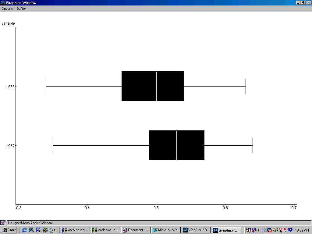
5. Statlets
Homework Problem:
Open Statlets, load the data. After speaking to the person who put down that they were 8’7" we found out that they actually wrote 5’7" but the 5 looked like an 8. Find this outlier in the data in the Statlets data screen and change 103.0" to 67.0".
1) What is the 95% confidence interval?
2) Then do a t-test on Ho: m = 68". Do we reject at 5%? Give another reason why you know this to be the case.
3) For what value of m would we not reject at 5%?
Solution:
1) Estimation of Population Mean for Height
Sample size = 45
Mean = 69.5111
95.0% confidence interval for mean:   69.5111 +/- 1.24635
                                                                  [68.2648,70.7575]
This means that 95.0% of all such intervals will contain the true mean.
2) t-test
Null hypothesis: mean = 68.0
Alt. hypothesis: not equal
Computed t-statistic = 2.44349
P-value = 0.0186264
Reject the null hypothesis for alpha = 0.05
Conclusion:
This table displays the result of a t-test performed to test the null hypothesis that the mean of the population from which the sample data come equals 68.0 versus the alternative hypothesis that the mean is not equal to 68.0. Since the P-value for this test is less than 0.05,we can reject the null hypothesis at the 95.0% confidence level.
Another reason: the 95.0% confidence interval for mean is at [68.2648,70.7575],and 68 is not in the range.
3) I think for a value which is between [68.2648,70.7575] would not be rejected. For example, we try Null hypothesis: mean = 69.0,and get the following result:
t-test:
Null hypothesis: mean = 69.0
Alt. hypothesis: not equal
Computed t-statistic = 0.826475
P-value = 0.412994
Do not reject the null hypothesis for alpha = 0.05