Advanced DEMs & Land Conservation
This lab is a joint effort between Joe Wheaton, Alan Kasprak, and Shannon Belmont
Here is your chance to dig into an important but often-overlooked characteristic of rasters: resolution. In this exercise we will explore the implications of resolution and elevation source material for visualizing, mapping, analyzing, and understanding landscapes.
We’ll be working with data from Monroe Mountain, Utah. Monroe Mountain is a sky island, or an isolated area of high-elevation terrain surrounded on all sides by lower elevation landscapes. Sky Islands, which are found across the Basin and Range of the Intermountain West and are also seen in the arid landscapes of Southern Arizona and New Mexico, are particularly important for wildlife and vegetation. That’s because the plants and animals found in sky island ecosystems are often “trapped” in those locations. They don’t have anywhere else to go, since they occupy the only high-elevation areas around. As climate warms, sky islands become particularly important refuges for these organisms, and they’re at risk of disappearing altogether.
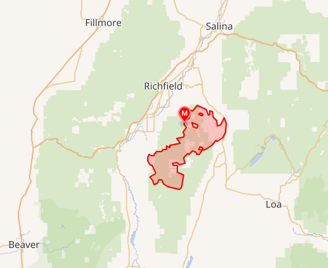
Update: A large fire burned approximately 300 sq km of Monroe Mountain in July of 2025.
Environmental impacts:
Burned soil after a fire can become hydrophobic, repelling water, which makes flash flooding more likely. That runoff can increase the risk of debris flows.
The Monroe Canyon Fire also impacted a lot of wildlife in the area. Thousands of animals, like deer, elk, and fish, depend on this habitat, and they’ll be dealing with food shortages.
Aquatic systems are affected too. Streams and lakes in the burn area support species like rainbow trout, Bonneville cutthroat trout, and tiger trout. After a fire, flooding can wash ash and sediment into these waterways, which can seriously impact water quality and fish survival.
Introduction

We are going to explore strengths and weaknesses of different resolutions and elevation source material. We will consider vertical and horizontal accuracy which is driven by the source material more than resolution.
You’ve landed a summer seasonal position as a GIS technician with the U.S. Forest Service, in the Richfield, Utah office of the Fishlake National Forest. The USFS is part of ongoing landscape restoration on Monroe Mountain, and so your supervisor has asked you to pull together some elevation data and make a map of the upper reaches of the mountain, along with doing some basic analysis on that data. The goal is to provide the partner agencies and landowners involved in the Monroe Mountain restoration project some information on which GIS data resolution is best for identifying causes of disturbance and sites for restoration on the Mountain. This group of stakeholders includes nonprofits, other federal agencies, private landowners, and the State of Utah’s Department of Natural Resources.
Getting Started
The first thing you’ll want to do is take stock of the DEMs, or digital elevation models, that you will access.
There are four products you’ll want to retrieve:
- 0.5 meter resolution lidar elevation models from the State of Utah
- 5 meter elevation models derived from photogrammetry from the State of Utah
- 10 meter elevation models from the USGS National Map
- 30 meter elevation models from the USGS National Map
So, let’s get started with obtaining some data! Then we’ll do some comparisons between the datasets and present our results to the stakeholder group.
Lidar DEMs from the Utah mapping portal
Head to the Utah Geospatial Resource Center, which is the state’s warehouse for all things GIS. Click on GIS Map Data, then Elevation. We’re going to download 0.5 m resolution DEMs from Monroe Mountain, so scroll down the list and find the relevant dataset from 2016. Click the View link.
Why do we care about vertical accuracy? Because we are downloading elevation data. Accuracy will inform our analysis and presentation of results.

Click on Retrieve 2016 Bare Earth DEMs and First Return DSMs via Interactive Map.
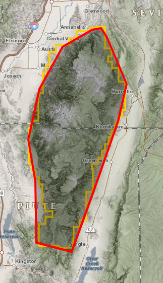
This will take you to a data retrieval map page. You’ll see the whole state of Utah displayed. Zoom in on the yellow polygon that represents Monroe Mountain. See below.
Once you’re there, you can use the polygon drawing tool to Define Area of Interest. It’s this one:


Draw a polygon around the lidar dataset boundary, clicking once to insert a point, and double clicking to end your polygon. The site seems to like it when you click your points slowly. If you mess up, you can just draw a new polygon to replace the first one.
Once you’re done, the site will automatically change the active panel in the table of contents to Step 3 - Results. Click on .5 Meter, then click Bare Earth DEM. Just so you know, the Bare Earth DEM will show the ground elevations, but the First Return DEM will be the first thing the laser beam, which is often shot from a plane, encounters first - it’s usually the top of the tree canopy.
Click Download. Then scroll down the list of DEMs and realize what a workload we’ve created.
You should also see the little blue tiles pop up on the map at this point, too. Each one of those tiles is an individual DEM file that you would need to download. I say would because we’re not actually going to download them all. The point here is to show you that lidar tiles are small because lidar files are big. Rather than providing one massive lidar DEM, Utah has cut them into tiles that are 42 MB in size each, so you can download individual areas more quickly.

If we wanted this whole area, we’d need to download more than 100 individual tiles, bring them into GIS, and mosaic them all together into one epic raster DEM. As we have other things to do with our lives, like eat and sleep, let’s not do that. Instead, we’re going to refine our area of interest to comprise only the very top of Monroe Mountain.
Click on Step 2 - Define Area of Interest again, and now draw a much smaller polygon that includes just the upper reaches of the highest part of the dataset. Here’s the general area we’re looking for. Try and match this as closely as you can. Make sure you get Signal Peak and Glenwood Mountain in there!


Now, same as above, click Results, Bare Earth DEM, Download. You should have at most four DEM tiles to download. Click the .zip hyperlink next to each of them to start each download. Save and unzip. If you don’t unzip them, you won’t be able to bring them into ArcGIS Pro.
Once the downloads are unzipped, add the files to your ArcGIS Pro project. If Arc wants to build pyramids, which help display the rasters more quickly, go ahead and do that.
Right-click on one of these DEMs > Properties, and become familiar with the coordinate system, file size, and bit depth of the data. This is 32 bit, floating point data with a cell size of 0.5 m and it’s projected in UTM, which uses units of meters. Make sense? Good!

This image shows 4 individual lidar tiles. Notice the maximum elevations for each tile in the contents pane. The tile in the upper right has a max elevation of 3280 meters. That elevation is drawn in white, which is the color at the high end of the color ramp applied to the range of elevations for each tile. The elevation tile to the south has a different range of elevation values. The white is applied to its highest elevation. That's why the colors disconnect at the tile borders.
Open and run the tool Mosaic to New Raster.
Use the raster properties to set up the tool correctly.
Demonstration of Mosaic to New Raster
So now we’ve got our 0.5 m lidar DEM. Let’s get some more data.
Photogrammetry Derived DEMs from Utah AGRC
Head back to the Utah AGRC homepage. Again, we want GIS Map Data and Elevation. All the way down at the bottom of that page, there’s a section on auto-correlated DEMs, which are produced from overlapping aerial images. In the same way that your eyes have depth perception because they provide slightly different views of the same thing, we can produce DEMs from photos taken at slightly different angles. The images used are from the National Agriculture Imagery Program (NAIP) which takes aerial photos during the agricultural growing seasons to assess plant crop health. In other words, most vegetation is at its fullest when these images are collected. And we use them to create elevation models of the ground. That there is some information that might be somewhat relevant later. The remote sensing class would spend a whole lecture on the process of photogrammetry, but for now, that’s the short story.
Click on Download 5 meter DEMs.
- Did you read the metadata?
- Did you see the bolded text in the paragraph introducing this data?
- Did you find the vertical accuracy?
- Did you catch that the 5 meter autocorrelated DEMs have a NSSDA (95%) vertical accuracy of 9.8 meters?
Same as before, you’re going to navigate to Monroe Mountain and download a similar area to the one you just grabbed for 0.5 m DEMs. You don’t have a yellow polygon to guide you, because these 5 m DEMs are available statewide and not just in certain areas. Zoom in to Monroe Mountain:

Just like before, draw a polygon to define your area of interest, and double click to end it. This will take you to the results, and then click 5 meter, Auto-Correlated DEM, Download. You’ll notice a blue extent indicator on your screen, which shows the tile you’re about to download. Because this data is coarser resolution, tiles of the roughly the same file size as before will cover a larger spatial extent.

Again, click the .zip hyperlink to download the data. Save it with your lidar data. Unzip.
Let’s take a second to talk about this new raster format, .asc, or ASCII, pronounced “ask-key”. It’s unique in that ASCIIs are one of only a couple raster file formats that are human-readable (’.txt’ being the other). That means you and I can open them and actually see the data outside of Arc. Double click the .asc file. Windows will probably have no idea how to open it, so select “More apps” and click Notepad or Wordpad or some other text editor that’s not MS Word. When it opens, you’ll see a bunch of text:

Let’s talk about these numbers:
- nrows is the number of rows in the whole raster; there are 4000 rows of data
- ncols is the number of columns in the whole raster; there are 4000 columns of data
- xllcenter is the x-coordinate (longitude or easting) of the center of the bottom left cell in the raster
- yllcenter is the y-coordinate (latitude or northing) of the center of the bottom left cell in the raster
- cellsize is well, the size of the cells in the raster; 5 m is what we’d expect here, right?
- NODATA_value is the value that’ll be used in the raster if a cell has no data. Here we’re using the common -9999 value, so if you see that anywhere in the matrix of numbers, you’ll know that cell has no data.
- And then all the numbers are the cell values themselves. In this case, it’s the elevation of the cells!
So let’s bring this thing into Arc.

- ArcGIS Pro doesn't refresh the view of your files automatically. Use the refresh button to 'see' data you have added to project folders post-connecting.
- If Pro still doesn't see your ascii file, change the data type to Raster (All Local Types).
- When adding rasters it is best practice to single click to select > Add / Open / OK
If you double click to open, you expose the bands that make up the raster. Ascii files only have 1 band, so you can double click and then add "band 1."
But for multiband rasters (like color imagery) adding the bands individually doesn't work.
Once you've added the 5 meter raster, go into the properties and examine the cell size, bit depth, file size, and pixel type.
Converting Ascii to Raster:
Search tools for "Copy Raster"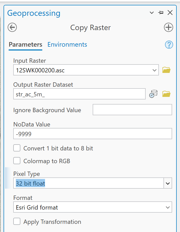
(The pixel type is found in the properties of the ascii file.)
BEFORE YOU RUN THE TOOL:
Go into the Environment Settings: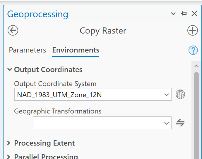
Set the coordinate system. Not sure which one? Check the webpage: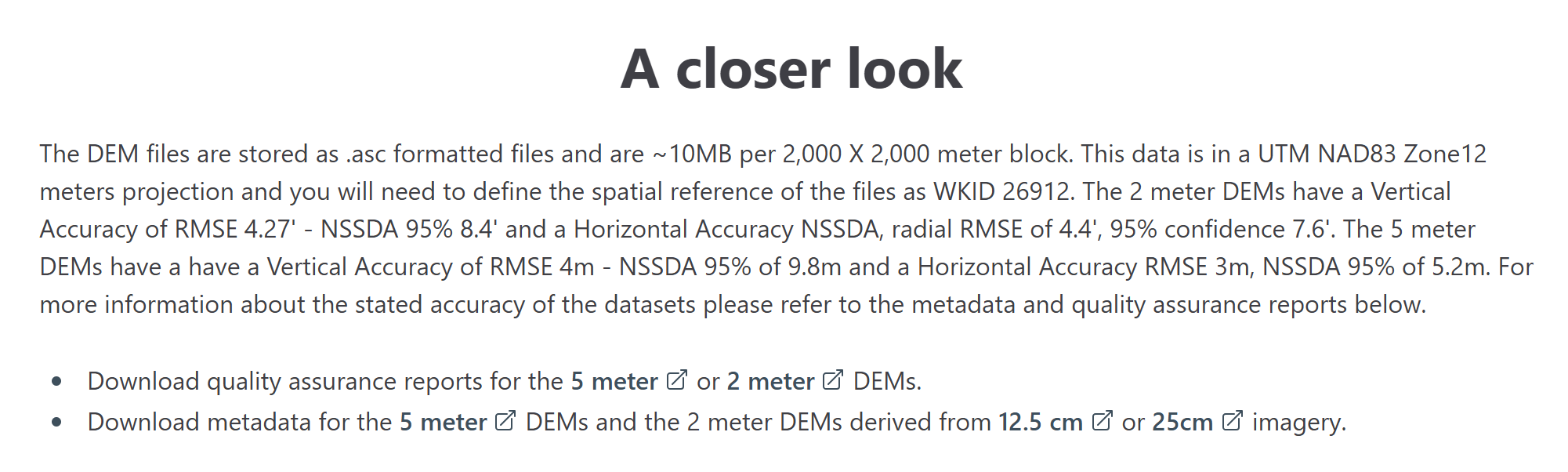
Side note on ASCII files and coordinate systems
ASCII files contain coordinate system information but ArcGIS doesn't have the capacity to read the metadata and create a projection file.
The other Environment setting is the resampling technique: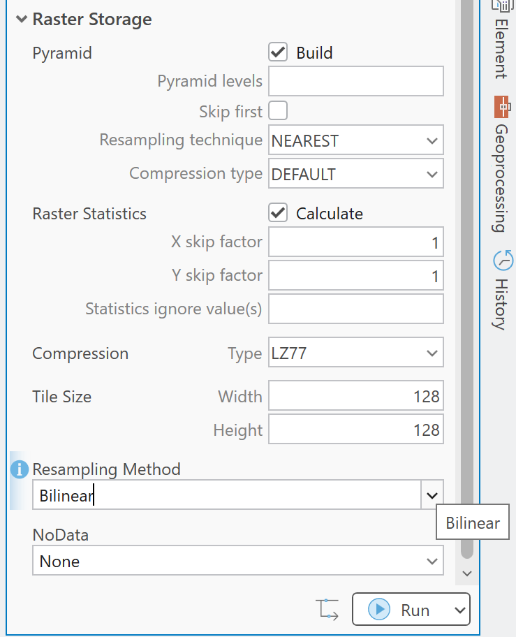
Run a hillshade from the 5m autocorrelated DEM.
Time for some housekeeping:
To keep things organized, consider grouping your layers in Arc.
To do that, hold CTRL and select the DEM and it's corresponding hillshade. With the layers you want grouped selected, right click and click Group. You can name this group something useful, like “0.5 m Lidar DEMs” (the names you assign in the contents pane are aliases and don't need to follow the same formatting rules as the original file). With layers grouped, you can turn the group’s visibility on or off with one click. If you want to, spend a second renaming layers and groups to get organized.

10 and 30 m DEMs from USGS National Map
Finally, you will download a 10 m and 30 m DEM of Monroe Mountain from the USGS National Map.
This is the place to be for “topographic information for the Nation.” You can also download hydrography data, watersheds, orthoimages, roads, geographic names, and land cover data for the US.
These DEMs are part of the National Elevation Dataset from the US Geological Survey and are derived originally from the contour data used to make the 7.5" USGS Topographic Maps. Elevation data is updated and improved when higher quality data can be incorporated.
Go to GIS Data Download and launch the data download application.
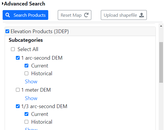
Check the box next to Elevation Products (3DEP).
- 10 meter data are called “1/3 arc-second” DEMs.
- 30 meter data are called "1 arc-second" DEMs.
Select them both.
When you’re downloading the 10 m DEM, the National Map will likely suggest two tiles for you to download, because Monroe Mountain happens to be right near the border of two big DEM tiles (because… of course it is). Don’t download both tiles. Instead, just choose the one that includes Signal Peak and Glenwood Mountain. Zoom in to find them on the map.
From the Datasets tab in the left pane, you will decide how to search and choose the products to search for.
- Zoom in to Monroe Mountain in UT.
- Use the Point tool to mark the Signal Peak location.
- In the lower section on the left, check the box for Elevation Products (3DEP).
- The 10 meter DEM is called “1/3 Arc Second.” Check that box.
- The 30 meter DEM is called “1 Arc Second.” Check that box.
Search Products
You can use the Footprint button in the results window to view the extent of the tiles to ensure you are grabbing the 10m tile with the peak.
- Click on “Download Link (TIF)” to download your tile.
- Add the 10 meter and 30 meter DEMs to your map.
Data Quick Check
At the end of all this, you should have 3 types of DEMs in your ArcPro contents pane (and 4 different resolutions):
- The 0.5 m lidar tiles (at most four of them)
- The 5 m autocorrelated DEM
- The 1/3 arc-second (10 m) National Elevation Dataset DEM (USGS)
- The 1 arc-second (30 m) National Elevation Dataset DEM (USGS)
Here's where you get your tuition's worth... Projecting DEM rasters
You should have noticed that the DEMs from the USGS national map came in a geographic coordinate system: NAD 1983. This makes sense because the data is national and the end use is unknown. Geographic coordinate systems are ‘general’ in nature, while projections are more specific; specific to the region and end use.
Before working with these geographic DEMs, they must be projected.
Run the tool “Project Raster”
- Use the browse button to navigate to your output file and rename your raster to something more descriptive: usgs10m
- Project to NAD 83 UTM Zone 12. Projected Coordinate Systems > UTM > NAD 1983 >
- NAD_1983_UTM_Zone_12N
- No geographic transformation is needed because the datum isn’t changing.
- Resampling Technique: Bilinear interpolation
- Cell size: this is a great opportunity to clean up the uneven measurement to an even 10 meters.
Run Project Raster for the 10 m and 30 m DEMs.

Project Raster requires that the raster cells are reorganized.
The tool allows the user to set the method for cell ‘sampling’. This is NOT an optional setting.
Don't accept the defaults!
Here's how to choose the correct resampling technique.
In the “resampling technique” section of the tool you should choose Bilinear for elevation data (continuous data). (Cubic Convolution works better for images.)
If you are working with discrete raster data (for example, Land Cover, where the cell values are codes that represent categorical data values) you would choose Nearest Neighbor.
Bilinear and Cubic techniques average between neighboring cells to create a smooth transition to the new cell layout. Nearest Neighbor takes the values from nearest neighbors to populate the new cell values.
You do not want ArcPro to average a cell value of 10 for open water and 70 for Aspen Forest because value 40 might represent urban, which makes no sense. But using nearest neighbor for continuous values creates artificial edges that wouldn’t normally occur on the surface.
Here's a video explaining the differences between resampling techniques:
Bilinear will process faster, cubic is a bit more computationally intensive.

If this happens to you - you didn't project your DEM before running hillshade.
To fix: go back and project your DEM into a projected coordinate system suitable for your area of interest.

This isn't just a bad look for your hillshades. These artifacts exist in the elevation model the hillshade was calculated from. The ridges can be so defined that they will interupt the way modeled "flow" behaves and create artificial ponding!
If this happens to you. Make sure you choose Bilinear as your resampling technique when projecting your DEM.
Then repeat the hillshade and delete all these bogus files you've manage to make. :)
Organize your data
At this point, you might consider grouping your lidar layers in Arc.
To do that, hold CTRL and select the lidar DEM and its hillshade - Right click > Group. You can name this group something good, like “0.5 m Lidar DEMs”. That way, you can just turn the whole group on or off with one click. Remove the individual tiles (pre-mosaic) from the map because you don't need them anymore.
Spend a second renaming layers and groups to get organized.
Group and rename the layers as needed (just click the layer names in the table of contents and give them a better name, like “10 m DEM” and “30 m DEM”).
Compare the Various DEMs
For this portion of the lab, we’re going to compare how each DEM represents elevations and do an exercise in drawing contour lines to see how these vary between DEMs as well.
Elevation of Signal Peak
Knowing elevations across the landscape can help prioritize areas for conservation; for example, on Monroe Mountain, aspens generally grow between 7,000 to 9,000 feet - but not all DEMs will show elevations equally! To demonstrate this, I’d like you to find the elevation of one of the highest peaks in the area, Signal Peak.
Load the SignalPeak.shp shapefile into ArcPro and bring it to the top of the layers (this shapefile came with the lab data this week).
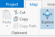
First, make the 0.5 m DEM the only visible DEM layer on the map. That is, un-check all the other DEMs, just leaving SignalPeak.shp and the 0.5 m DEM underneath it visible. Zoom in to the point marking the summit of Signal Peak, and use the Explore tool (in the Map tab) to click on the point.
If you clicked the Signal Peak point, it’ll show a value of “0” or "1" in the explore tool pop-up window. That's the feature ID for that point, which isn't very interesting. We want to know the value of the underlying DEM. Under Explore, click the drop-down arrow and tell it to use Visible Layers. Now click the point again.
Demonstration of the Explore Tool:
- That’s more like it! Note the elevations of Signal Peak stored in each of the datasets.
- Explore other areas as well, like ravine bottoms or steep slopes.
- Are there some datasets that are more similar? More different? It might be interesting to calculate the differences between one dataset and the others and make a table.
- How much do the elevations vary?
- Think about why the elevations vary so you can make brilliant observations in your write up.
Contour Lines to compare DEMs
Finally, let’s create contours from the DEMs.
Using the Contour tool (search for it), input your 0.5 m DEM for the Input Raster. You might need to select just one of the tiles if you have multiple ones, so turn the individual tiles on and off to figure out which one contains Signal Peak. Use that one for the contouring.
Choose a good name for your contour lines, which will be a polyline. Something like “Contours05m”. Make the contour interval 10 m (this is the elevation difference between consecutive contour lines). Set the Base Contour to 2700 (this is an elevation near the minimum elevation of the smaller extent of the lidar tile). Leave everything else as it is, and hit Run.
This should export some nice-looking contour lines!


Create contours from other elevation models as you see fit
Think about how you can use the generated contours to illustrate the difference between the datasets.
Hillshading
Although DEMs are very useful, by themselves raster DEMs don't automatically display the topography in a way that makes the terrain jump out at you. It turns out that the visual context we like from DEMs is best provided by a product derived from the DEM - a hillshade. In fact, DEMs are rarely (if ever) displayed without its corresponding Hillshade.
Starting with the lidar elevation data, open and run the hillshade tool on it.
Naming strategy: I like to name my hillshades so that they are always found with their corresponding DEMs in my files.
Examples:
- DEM name = monroe_5m
- Hillshade name = monroe_5m_hs
Hillshades are unique to the elevation data they are derived from.
You must create a unique hillshade from each DEM you have.
Helpful Reminders and Discovered Work-Arounds:
- Don't put color ramps on hillshade (color ramps go on elevation layers)
- Raster file names still cannot contain more than 13 characters
- Those characters must be alphanumeric except for our dear_friend_the_underscore.
- This is also true for files located anywhere along the raster file's path.
- C:\Users\Default 2\App Data = NO
- C:\Users\Default2\AppData = YES
- Don't start your raster file or folder names with numbers
- 5m_DEM = NO
- DEM_5m = YES
- 999999: Something unexpected caused the tool to fail.
- This is most often (in my experience) caused by a bad file name or a space in the file's path
- Try saving your output to the desktop (creates a clean path) and make sure you follow the rules above.
- You will need each of your rasters in their own map for the layout. (i.e. not 4 map frames referencing the same map)
- Use the cylinder in the contents pane to list your layers by their source location
properties source for file's real name - If your hillshade is drawing with dark shadows despite having projected your DEM, experiment with the symbology 'Stretch Type' settings:

Additional Resources
- How to match the scale and extent of each map frame & matching color ramps!
- How to clean up a scale bar
- How to create a beautiful elevation legend