Antarctic Ice Sheets and Calculating Sea-Level Rise
Overview
In this lab, you will explore the Bedmap2 dataset and investigate how Antarctica might appear if its ice sheet were removed. Using raster analysis tools in ArcGIS Pro, you will create three map products that visualize Antarctic bedrock under different sea-level scenarios.
The core content of this lab was originally developed by Mark Helper for GEO 326G/386G: GIS & GPS Applications in Earth Sciences offered in the Department of Geological Sciences at The University of Texas at Austin. The original material has been modified and supplemented with advanced tasks. Used by permission.
Lab objectives and Skills
By completing this lab, you will be able to:
- Visualize and interpret raster elevation datasets.
- Apply raster symbology techniques to improve terrain visualization.
- Use Raster Calculator, Reclassify, and Contour tools.
- Model isostatic rebound following ice-sheet removal.
- Evaluate the effects of sea-level change on continental landforms.
- Critically assess assumptions and limitations in geospatial modeling.
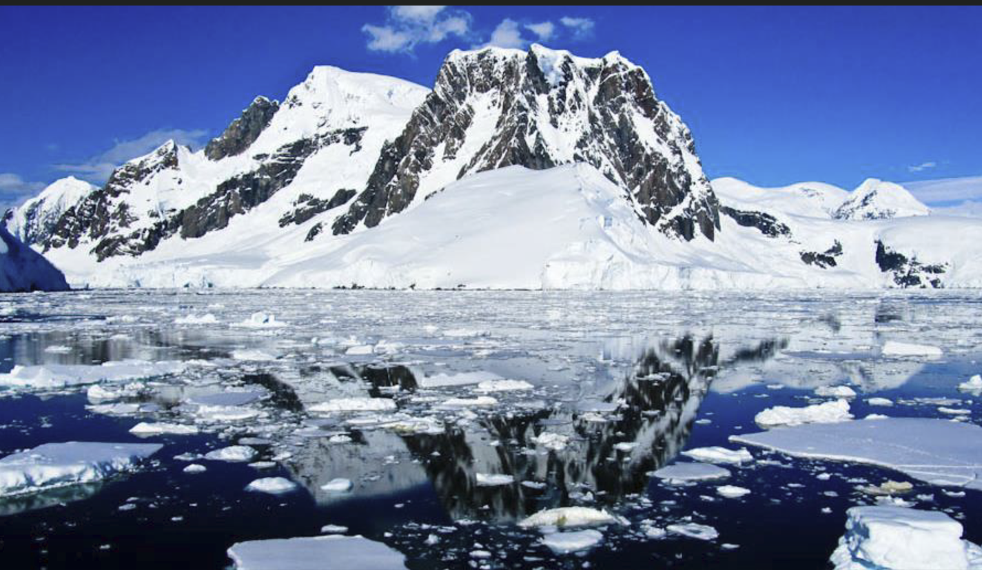
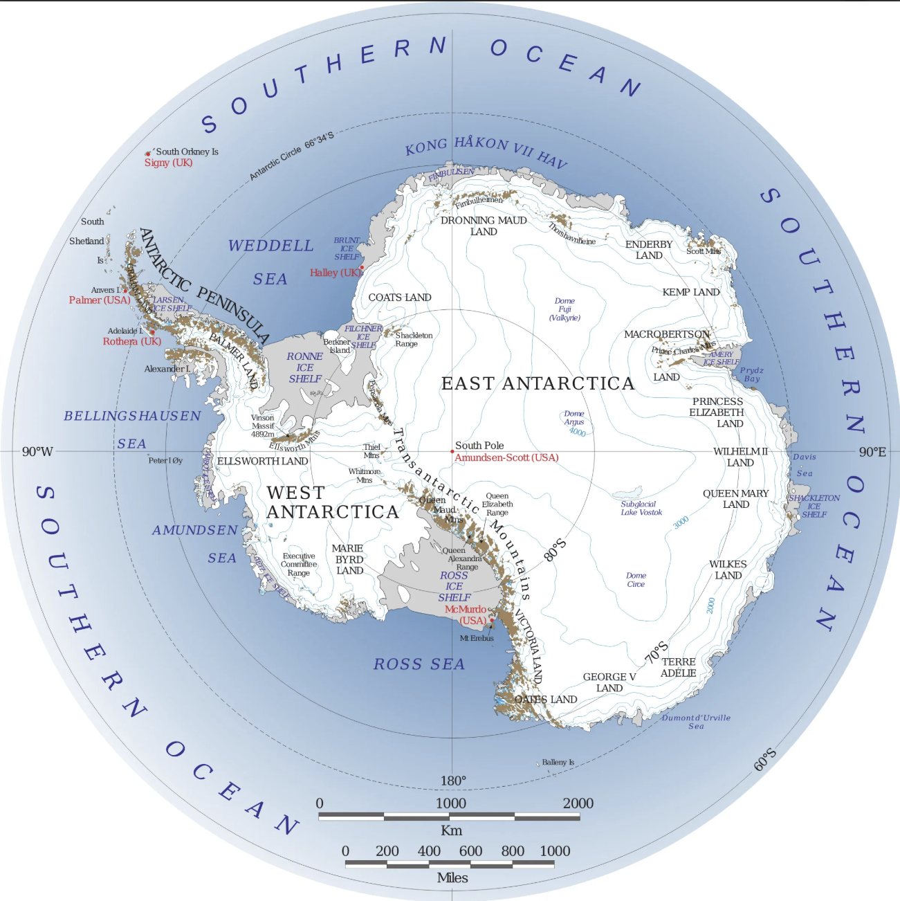
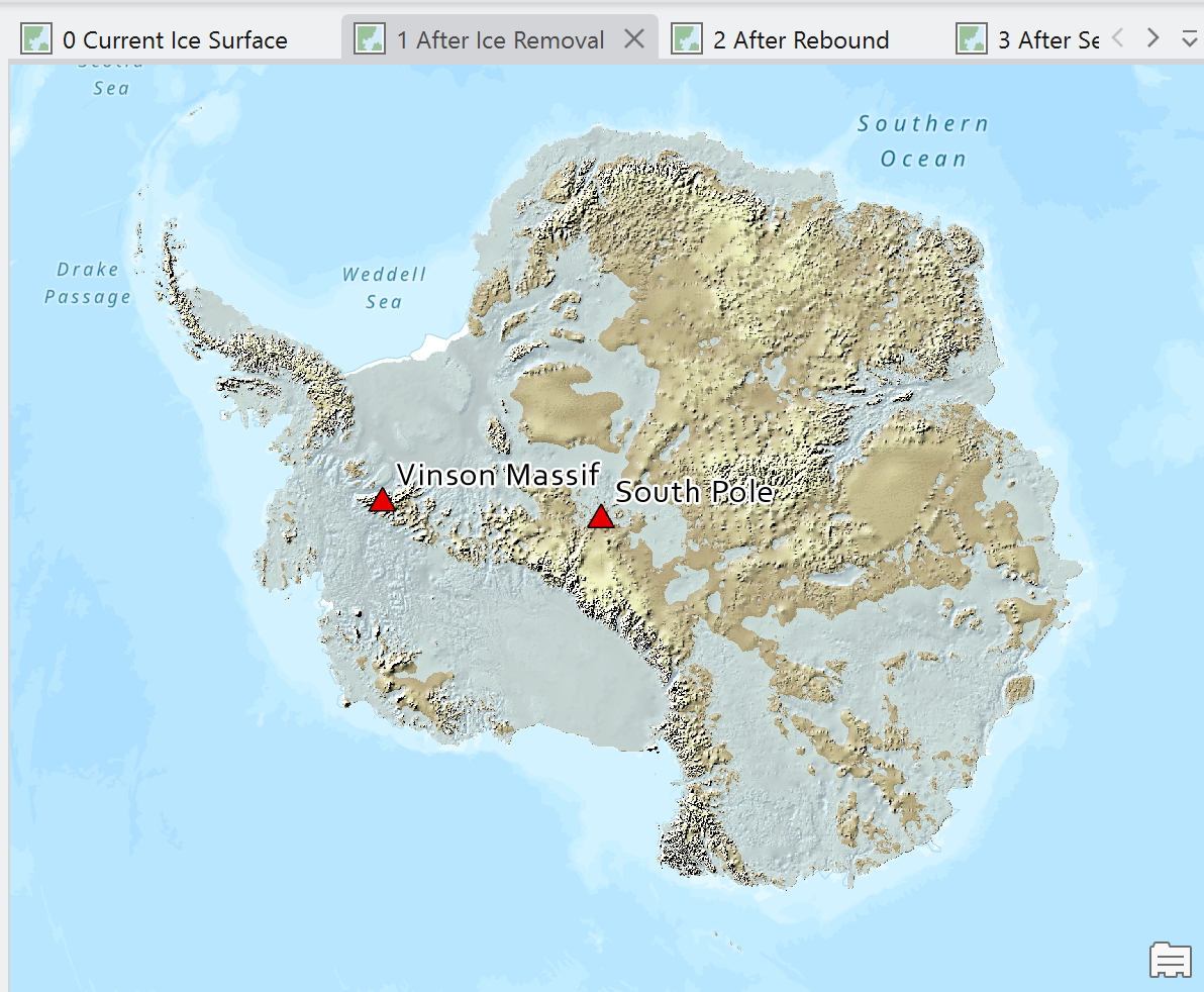
What does Antarctica look like beneath the ice? A continent of mountain ranges, deep valleys, plains, inland seas, and offshore islands exist there. But they are invisible for the most part except for a few features that protrude above the ice. It would be an interesting visualization tool to have a topographic map in shaded relief of Antarctica with the ice removed and with oceans filling areas that are below sea level. It might be more informative if that map that accounted for the isostatic rise of the land surface that would occur after the weight of the ice was removed and sea level was adjusted to include the volume of water locked up as ice. Remarkably, digital data now exist to make such maps and answers these questions, and we have the software needed to do so.
Part 1: Project Setup and Data Exploration
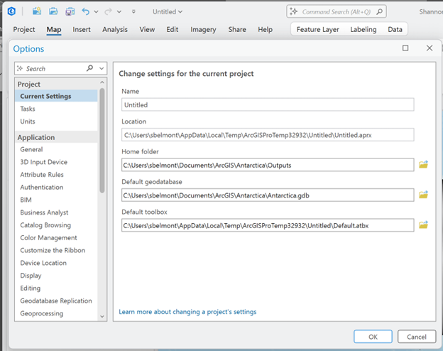
Create a New Project
1. Create a new ArcGIS Pro Project
2. Create and assign:
- a dedicated Home Folder
- a dedicated Default Geodatabase
- Project > Options > Current Settings
Add Data to a new map.
Data recap:
The data comes from the Antarctic BEDMAP2 project.
https://www.bas.ac.uk/project/bedmap-2/
- Bedmap2 was published in 2013.
- Bedmap3 began development in 2020 and is still underway.
BEDMAP provides rasters of Antarctic bedrock elevation and adjacent ocean floor bathymetry, of Antarctic ice thickness, and of Antarctic surface elevations.
Layer descriptions:
|
Bed2_surf |
Antarctic surface elevations (ice surface) |
|
Bed2_surf_hs |
Hillshade of surface elevations |
|
Bed2_bed |
Bedrock elevations beneath the ice |
|
Bed2_bed_hs |
Hillshade of bedrock elevations |
|
Bedmap2_thickness |
Estimated ice-sheet thickness |
|
Pts_of_interest |
South Pole and Mt. Vinson locations |
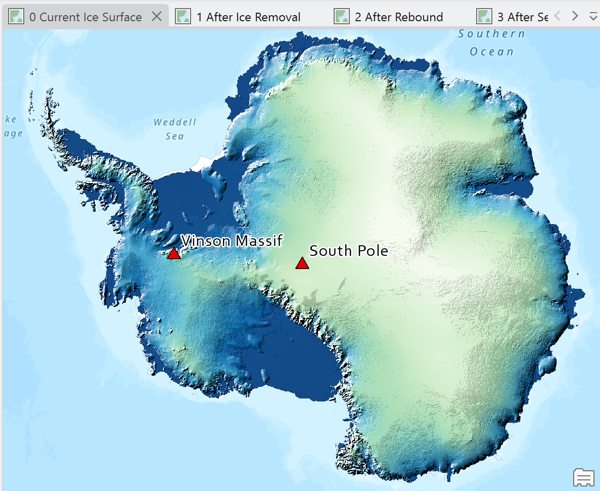
Part 2: Visualizing Current Ice Surface Elevations
Ice Surface Symbology
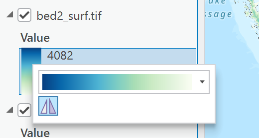
- Open the Bed2_surf layer.
- Apply a continuous elevation color ramp (ex. Green-Blue Continuous)
- Ensure the color ramp follows standard elevation conventions:
- Light colors = high elevations
- Dark colors = low elevations
- Reverse the color ramp if necessary.
Examine the ice surface hillshade
The default hillshade appears relatively flat because elevation variation is subtle across much of the Antarctic ice sheet.
- Open Bed2_surf_hs symbology.
- Change Stretch Type to:
-
- Standard Deviation
- 2 standard deviations
This technique often improves visualization of landscapes with limited relief.
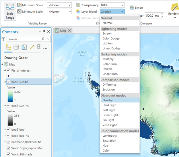
Create a Blended Terrain Visualization
- Select the Bed2_surf layer.
- Under the Raster Layer tab:
-
- Set Layer Blend Mode = Overlay
This technique often improves visualization of landscapes with limited relief.
The layer is blended with the layer visible below it in the contents pane. The elevation raster needs to be listed above the hillshade in the contents pane and both need to be visible.
What is the highest elevation in the Bedmap2 Ice Surface Elevation dataset?
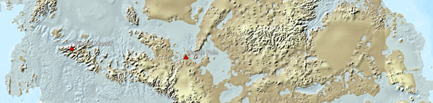
What is the elevation of the ice surface at the south pole?
(The south pole is one of the two points in the Pts_of_interest layer.)
Part 3: Exploring Bedrock Elevation
Turn off the ice surface layers and examine:
- Bed2_bed
- Bed2_bed_hs
Mt. Vinson is the highest mountain in Antarctica.
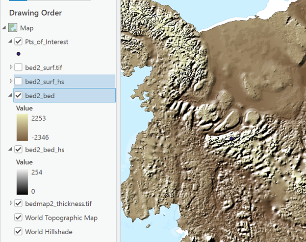
Using the Bed2_bed layer:
What is the bedrock elevation at Mt. Vinson?
(Mt. Vinson is one of the two points in the Pts_of_interest layer.)
Why do you think this elevation is lower than the maximum elevation observed in the ice surface elevation dataset?
Research the generally accepted elevation of Mt. Vinson and compare it to your measurements.
Write a short observation comparing the BedMap2 elevation of Mt Vinson and the generally accepted elevation of Mt Vinson. Which is higher? What are some explanations for this this difference in elevation?
Analysis Goal
You will create three map products:
Map 1: Antarctic bedrock with current sea level. Ice cap is magically removed and held temporarily in an intergalactic space.
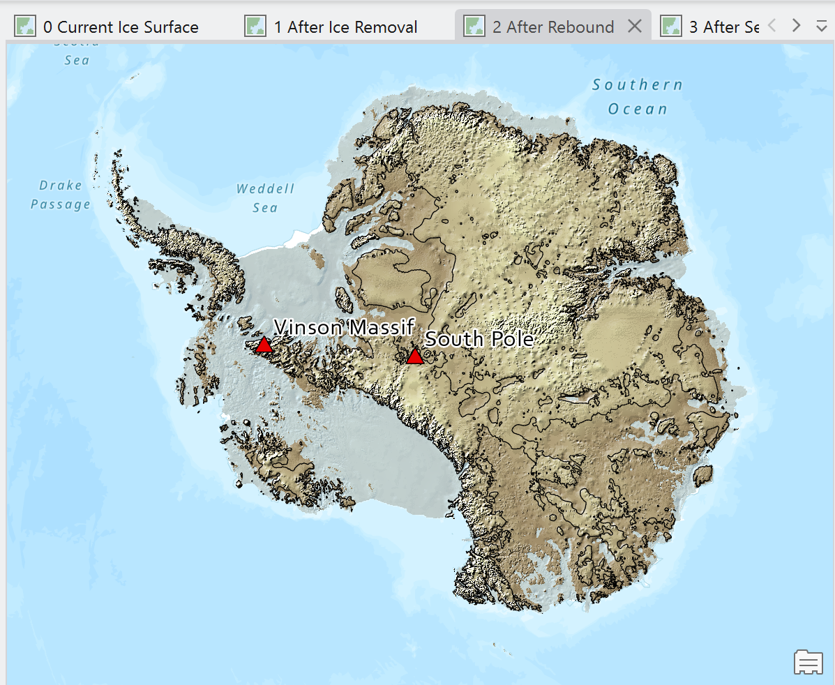
Map 2: Antarctic bedrock after the continent is allowed to react (bouy) to ice cap removal.
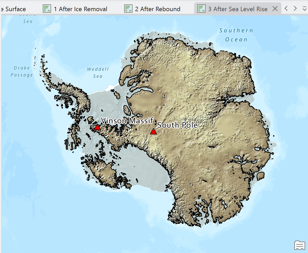
Map 3: Antarctic bedrock after rebound with sea level increased by melting all global ice.
Part 4: Map Product 1 - Bedrock with Current Sea Level
Prepare Layers
Turn off all layers except:
- Bed2_bed
- Bed2_bed_hs
Create a Sea Level Layer
Use the Reclassify tool.
Input Raster: Bed2_bed
Classify Elevations
|
> 0 m |
New Value = NODATA |
|
≤ 0 m |
New Value = “1” |
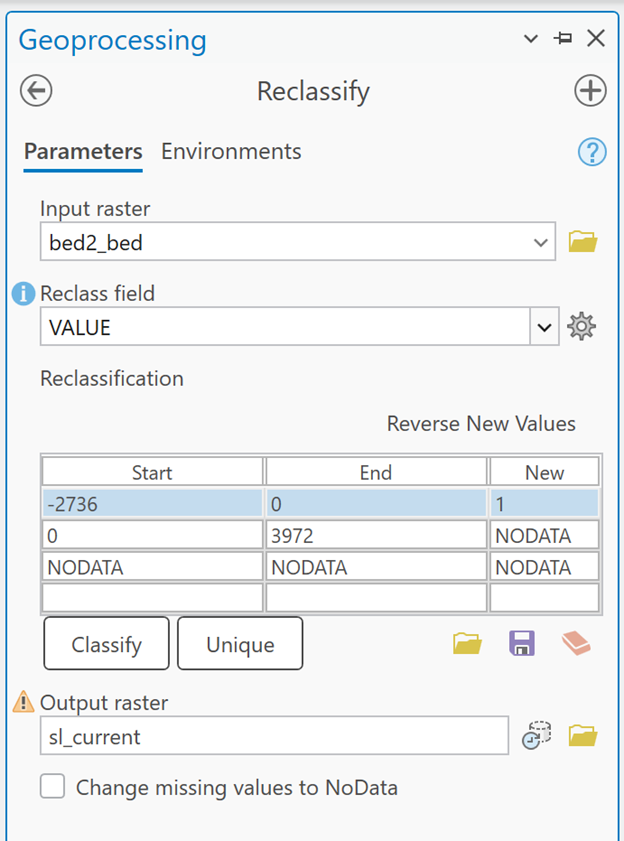
Save as: sl_current
(for sea level – current) (You can save it as whatever you want. But HEED THIS: you will want to name your outputs very carefully. This is going to get messy fast. Sl_current is what I will be referring to this output layer as going forward.)
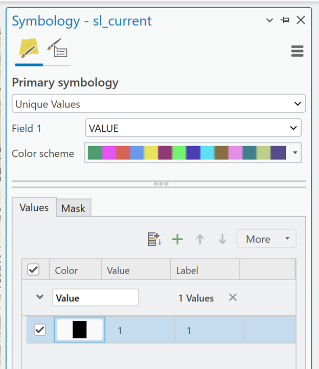
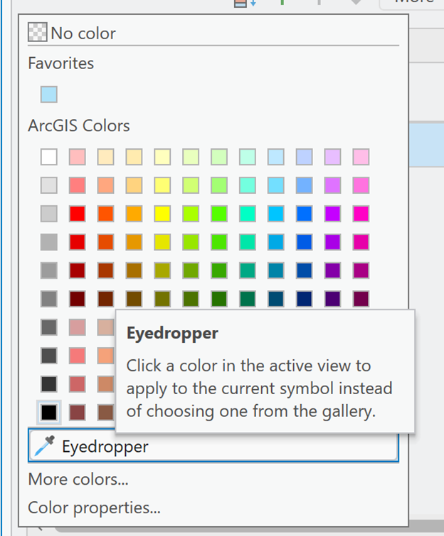
Symbolize Sea Level Areas
- Change the raster color to match the surrounding ocean using the eyedropper.
- Set transparency to approximately 50%.
What is the estimated bedrock elevation at the South Pole?
Create a Sea Level Contour
Use the Contour tool.
This will be used for cartographic purposes. A thin line representing where sea level is on the landscape.
Parameters
- Input Raster: Bed2_bed
- Base Contour: 0 m
- Contour Interval: 4500 m
Why 4500 meters? This means there will be an initial contour at 0 m elevation (sea level) and then another one at 4500 meters elevation. 4500 meters exceed the max elevation of the continent. This produces a single contour representing present-day sea level.
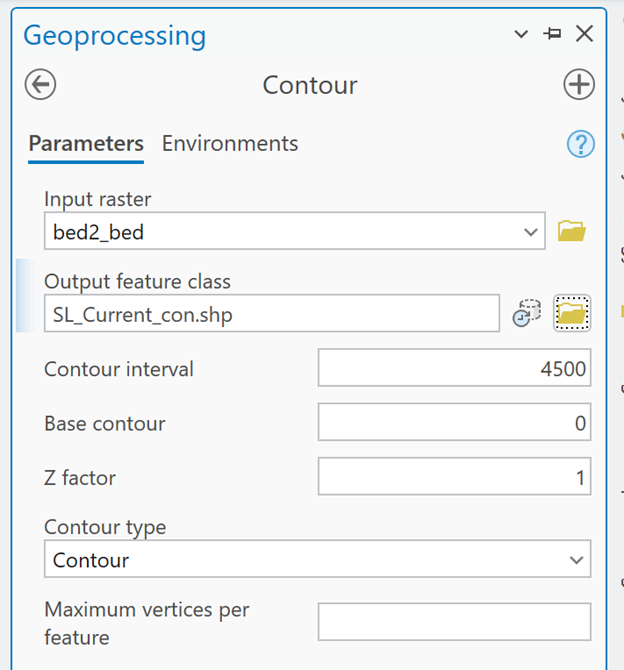
Save as: SL_Current_con (for sea level, current, contour)
Part 5: Map Product 2 - Accounting for Isostatic Rebound
Background
When a large ice sheet is removed, the crust rebounds upward due to the reduction in weight.
The rebound amount can be estimated as:
Elevation Change = (Density of Ice) / (Density of Mantle) * (Ice Thickness)
Assume:
- Ice density = 0.98 g/cm³
- Mantle density = 3.34 g/cm³
Density ratio:
0.98/3.34 = 0.2825
Calculate Rebound
Use Raster Calculator:
Amount of Rebound = Bedmap2_thickness × 0.2825
Save as: Rebound_amt
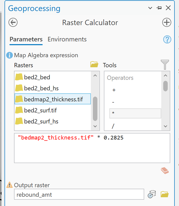
The resulting raster will represent the amount if elevation change at each cell’s location due to the rebounding of the continental bedrock after removing the weight of the icecap.
Depending on the varying ice thickness, the continent will rebound different amounts at different locations.
Amaze
Amaze
Amaze
What is the estimated maximum amount an area of the continent would rebound (rise)?
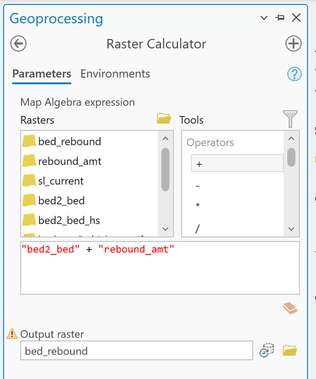
Create Rebounded Bedrock Elevation Layer
Use Raster Calculator:
Bed_Rebound = Bed2_bed + Rebound_amt
Save as: Bed_rebound
If some areas rebounded as much as you reported in Question 7, is this new maximum elevation value what you would expect? Why or why not?
What is the new elevation at the South Pole after rebound?
Create Supporting Layers
Hillshade
Create a hillshade from Bed_Rebound.
Recommended stretch: Standard Deviation
Symbology
Apply the same color scheme used for previous bedrock maps.
Set Layer Blend Mode = Overlay with elevation above hillshade in the contents pane.
Sea-Level Contour
Create a 0-meter contour from Bed_Rebound.
Sea Level Visual
Reclassify the Bed_Rebound as before.
NODATA for elevations above sea level, “1” for elevations below sea level
Use the same ocean color and transparency as before.
Part 6: Map Product 3 - Rebounded Elevations with Global Sea Level Rise
Background
Removing Antarctica's ice would raise global sea level by approximately 73 meters.
Removing all ice on Earth would raise sea level by approximately 80.5 meters.
To model this scenario, adjust elevations relative to a sea level that is 80.5 meters higher than today.
Create Adjusted Elevation Surface
The elevations aren’t “moving” like they did with rebound. Instead, we are using the raster calculator to ‘reset’ elevations relative to a new sea level.
Use Raster Calculator:
Bed_Rebound − 80.5 = Bed_rbnd_slr (for rebounded bedrock with sea level rise)
Create Supporting Layers
Only one is needed.
Sea-Level Visual
- Reclassify
- Same ocean color as before
- 50% transparency
Deliverables
Map Layout
Create a layout containing all three map products side-by-side.
Requirements:
- Same map extent
- Same scale
- Same-sized and proportioned map frames
- Consistent symbology
- Consistent color schemes, transparency, and blend modes
- Appropriate and descriptive titles and context
For each map, report:
- South Pole elevation
- Bedrock and Sea-level condition represented
Written Reflection
Submit a brief write-up addressing:
Workflow Challenges
- What difficulties did you encounter?
- How did you overcome them?
Critique of the Analysis
- What assumptions are being made?
- What limitations exist in this workflow?
- How could the workflow be improved?
Data Evaluation
Discuss:
- Data quality
- Accuracy
- Precision
- Resolution
- Sources of uncertainty
Scientific Observations
Describe any interesting geographic or geomorphic patterns revealed by the analysis.