Case Study: Watershed Delineation

The Basics

In this exercise you will calculate new surfaces from digital elevation models that can be used to generate stream networks. The resulting networks are dependent on the quality of the elevation data used to originate the derivative surfaces. As you work through the exercise, think about the data in reference to the uncertainty principles previously discussed.

While these steps have a hydrologic slant to them, remember that the skills in this lab are fundamental to any type of raster analysis you may otherwise undertake. Think about how you could apply these same tools and functions to other problems.

Figure 1: Shaded relief map showing the Caspar Creek Experimental Watersheds and the surrounding region. A Field-Based Experiment on the Influence of Stand Density Reduction on Watershed Processes at the Caspar Creek Experimental Watersheds in Northern California Dymond, Salli et.al. 2021

Lab objectives

The lab not only gives you experience working with DEMs, but many of the skills you develop here are more generally applicable to dealing with raster datasets in general. In this exercise you will:

1. Download a DEM in an area of interest
2. Delineate a watershed
3. Use flow accumulation to approximate a stream network
4. Calculate stream order
5. Summarize and compare landscape characteristics within neighboring watersheds

Data Download

Download a 10m DEM from the USGS National Map. You will need to download an extent large enough to cover an entire watershed (typically 1-2 tiles). Watersheds differ in size, so choosing the pour point will be a critical step. Review the lecture content for details about pour points and visually identifying watershed. If you need instructions for downloading DEMs, revisit the DEM Mastery lab.

Here's a quick introduction to pour points and an ideal landscape for this week's analysis:

You can choose any area in the United States that has an available 10 meter DEM. Try to avoid areas with a lot of lakes or a big reservoir. 

If you choose a relatively flat area, your contributing area could end up being quite large. You may need to mosaic several tiles to cover it all (and it may be difficult to visually determine the drainage divides of the watershed).

Suggestions

Don’t be a hero. Keep your watershed small and easily identifiable. Ideally, one 10m DEM tile is sufficient. If you over-reach and try to model the Mississippi River basin… you will spend days waiting for each tool to run. Working in an area with obvious drainage divides will help. You need to be able to visually verify your full watershed is covered by the DEM tile(s).

If prompted to do so, you will find these (and all) rasters will display quicker if you Build Pyramids for them. If you aren’t familiar, building pyramids improves display performance and is - generally speaking - a good idea.

Tools You Might Need

...to get your data prepped:

• Mosaic to new raster: if you want to stitch multiple DEM tiles together
• Copy Raster: if you are working with an ascii file
• Define Projection: if your data has no projection file (the coordinate system is undefined)
• Project Raster: if your data is in a geographic coordinate system, you need to project it. (Data from the USGS needs to be projected.)

Add your DEM data to Arc and evaluate the extent and general ‘correctness’ of the data (does it load, draw, have an appropriate range of elevation values displayed in the table of contents?).

If necessary, run Project Raster to transform the DEM's geographic coordinate system to a projected coordinate system appropriate for your area.

If you aren't sure which coordinate system is right for your area of interest, you can Google it.

Also, the State Plane coordinate systems are easy to use as they include the state name in the description.

You can also Google maps of the UTM system to find out which UTM zone your data are in.

 

Data Prep- fill, flow direction, flow accumulation

This part of the exercise will utilize a sequence of tools to generate a series of output raster surfaces derived from your elevation model. Watershed delineation requires the following series of steps:

Fill - Repair holes or sinks in the DEM that might interfere with modeling flow on the surface

Flow Direction - Calculates the direction of ‘flow’ for every cell given the elevation of the neighboring cells – output values represent the direction of theoretical flow across each cell). Use the Filled DEM as input.

Flow Accumulation – Calculates how many cells would ‘drain’ into any given cell – output cell values represent the number of cells in the raster that drain into that cell. Use the Flow Direction as your input.

Flow accumulation is used primarily for 2 things in this workflow:

• a way to visualize the correct cell for your pour point
• reclassify the values to create an estimated channel network (part 3)

Flow accumulation is an interesting raster surface to think about. If a cell has no cells flowing into it, that defines a drainage divide or ridge.

Snap Pour Point: ensures that the outlet location defining your watershed is coincident with the flow accumulation ‘channel’. This tool isn’t necessary when you are delineating 1 watershed. But when you are automating the process to delineate hundreds of watersheds, it is critical to have a tool that can move points to coincide with nearby cells that have the highest flow accumulation to ensure correct delineation.

Watershed Delineation tool - Creates a very simple output containing all the cells that drain into a designated cell – marked by the pour point – output value typically “0”. The output cells define the watershed or contributing area for the pour point.

 

 

As we move forward, please be very careful about how you name your data. Here are some suggestions so you don’t get mixed up. Remember, no spaces, no special characters other than "_", and raster files can't start with a number.

In this example, we are using a 10 meter DEM from the USGS. Let's call it "USGS10m"

• DEM = usgs10m (raster files can’t start with a number)
• Fill output = usgs10m_f
• Flow accumulation output = usgs10m_fa
• Flow direction output = usgs10m_fd
• Hillshade = usgs10m_hs
• Reclassify = usgs10m_rc

Using the same 'root' for all DEM derivatives ensures that all the layers will be stored together alphabetically in your files.

 

 

Get Started

 

Run the Fill tool on your DEM and name the output.

Run the Flow Direction tool using the Filled DEM as the input. (Use D8 as the type)

 

 

Run the Flow Accumulation tool using the Flow Direction raster as the input and Output type integer. This tool takes a while to run, so maybe go take a break now. If it takes too long to run, try clipping your raster to a smaller area, or only using one tile.

 

 

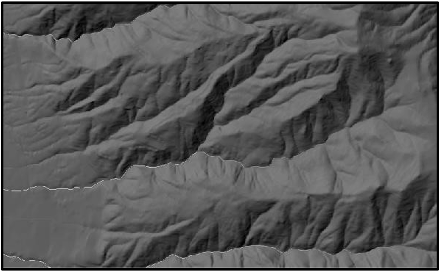
Here is what a portion of your Flow Accumulation layer might look like:

If your flow accumulation layer doesn’t look like this, zoom in. There aren’t a lot of cells in the high end of the range of values… and the cells are small.

Zoom in to verify. Try displaying using Standard Deviation (Symbology > Stretch Type= Standard Deviation > 2 StDevs).

 

 

Notice the range of Flow Accumulation values in the table of contents. Remind yourself: What do these values tell us about the raster? Use the explore tool to sample individual cells. For context, display the flow accumulation over a hillshade layer or basemap so you can see the terrain.

The cell values represent the number of cells draining into any given cell. So where would you expect the highest valued cells to be located in the image above if the legend tells us that black = low values and white = high values? How do these values relate to elevation? The high value itself will depend on the raster extent and resolution. The cell containing the highest number of other cells that drain into it will be near the downstream side of the DEM.

Verify that the flow accumulation lines are continuous. Zoom in on the white cell lines to verify that they don’t have gaps where you'd expect flow to continue. Gaps would imply that the DEM wasn’t filled properly. See the gaps in the image above? That’s from the screen resolution. Zoom in and you’ll see they are continuous. But sometimes they aren’t. If the lines are truly discontinuous, rerun Fill and repeat the steps up to this point. Or make sure you used the filled DEM when you ran flow direction.

 

Choosing a Pour Point

A Pour Point is the output of the watershed. It is the one place to which all the water uphill flows. Use the flow accumulation raster overlaid on a hillshade to look for basins (enclosed watershed areas). You might want to place the pour point near a canyon or basin entrance. There isn’t a “correct” location to define where a watershed starts.

Whatever point you choose, the tools will find the area that “contributes” or flows to that cell.

Try changing the symbology of the flow accumulation raster so you can see more of the flow network. The easiest way to do this is to set the stretch type to histogram- equalize.

To get a display like this, change the display transparency of the Flow Accumulation layer to 50% and display above a hillshade.

You can also use the Appearance tab to Blend the flow accumulation layer with the hillshade.

 

Create a point feature

Creating a point:

There are a couple of ways you can do this. 

One way is to digitize a point into a shapefile.
Another is to create a graphic point (like a drawing) then convert it to a shapefile.

The Digitizing workflow is summarized like this:

• Create a new empty shapefile, designate it as a point file, and assign it to the correct coordinate system for your area of interest.
• In Edit, Create a New Feature, Draw your point.
• Save your edits.

The Graphics workflow is summarized like this:

• Insert a graphics layer 
• Draw your point
• Run "Graphics to Feature" to convert the drawing to a shapefile
  • Use the Environment settings to assign a coordinate system to the output feature.

Video Demonstration of the Graphic workflow:

 

 Digitizing Instructions:

1. Create an empty point file in your data folder.
   
   • In Catalog: right click on the folder > New > Shapefile
   • Make sure it is a point file. 
   • Template, Has M, Has Z, Feature class alias and geodatabase settings can be left as-is.
2. Edit
   • Select your pour point layer in Contents pane
   • Edit tab on the main ribbon > Features > Create
   • Select your layer in the Create Features window to access the add point tool

Video Demonstration: Creating a pour point by digitizing

 

 

Zoom way in on your flow accumulation line near the mouth/lowest point of your watershed and click inside a white flow accumulation cell to add a point. Get your point ON the flow accumulation line.

SAVE YOUR EDITS

 

 

In the image below, notice the different pour point loctions and the adjustments to the upstream contributing areas.

The raster tile above isn't big enough data to map the full watershed estimated by the crossed out pour point and sketched in with the orange dashed line. In reality, the watershed tool would return a watershed with an abrupt horizontal and vertical straight edge. We don't have any information about what happens off the raster tile, so that pour point location (with the red X) is inappropriate.

If you run the watershed tool and get a straight edge, the tool isn't capturing the full watershed.
Edit your point location: moving it up a tributary off the main channel. You should be able to visually trace the outline of the full contributing area using the ridges or drainage divides.

 

Recap

At this point you have:

• A flow accumulation raster
• A point that defines the downstream ‘outlet’ of whatever basin you intend to define.

 

Delineate the Watershed

Find and Run the Watershed tool in the toolbox, not the ready-to-use tools.

Notice that it prompts you to input the Flow Direction raster.

Best practice naming convention: designate that it was created from the 10m data (i.e. dem_name_ws).

Evaluate the results. Does the watershed extend to the ridgelines as you expected or predicted?

 

 

Prepare for next steps

 

Run the Raster to Polygon tool to create a polygon version of the watershed.

Clip your flow accumulation raster using this polygon using the Extract by Mask tool or the Clip Raster tool.

 

Why clip the flow accumulation raster? Because you will be running the stream order tool, which is a global function, meaning it takes the full raster into consideration. You only want to calculate stream orders of the channel in your watershed relative to itself.

Estimating the Stream Network

...from Flow Accumulation

 

Open the symbology of your clipped flow accumulation layer.

 

Now you will use the flow accumulation layer to create a map of the channel network.

This is done by classifying (simplifying) the continuous range of flow accumulations values down to 2 classes: "stream" and "not stream"

Do high or low accumulation values represent areas of the landscape that might collect actual running water?

 

 

Change the Primary Symbology to classified.

Create 2 classes and set the break value fairly low to make the accumulation values easier to see.

Read on.

 

Find a flow accumulation value that allows you to visualize a reasonable stream network for your watershed.

 

Finding the threshold

In the series of images, the blue line represents the watershed boundary. The headwaters would be to the east, water flowing to the west. Notice as the threshold value decreases, the white channel line moves up into the headwaters and tributaries form.

 

What accumulation value gives you the most realistic looking stream network?

Experiment using the symbology classification tools to visualize the resulting 'network' using different threshold values.

This is a good way to estimate where to divide the range of flow accumulation values to create two classes before running the Reclassify tool.

 

Compare your classes to a basemap

• USGS National Map has data on where streams can be found. Be aware that even this USGS map isn’t 100% accurate.

Or compare your network to the NHD stream polyline data from the USGS

• or the Utah mapping portal has USGS stream polylines ready to download if you are working in Utah.

 

 

How well does your “stream network” match the mapped stream network? You may need to zoom in and pan around to explore.

Keep changing the break value until your “stream network” roughly matches the USGS network. It won’t be perfect, but get as close as you can.

Reclassify

 

Once you have your threshold value dialed in, run the Reclassify tool.

For the stream order tool to run correctly, delete all cells in the class of low accumulation values.

• Low flow accumulation class values >> New Value = NODATA
• High FA values > New Value = 1

Remember, raster file names are limited to 13 characters. No spaces!

A reclassify of flow accumulation at 500 cells would look something like this:

 

 

Evaluate your results. You should have a raster that only has cells in the channel line; a raster with only one value and a lot of areas with No Data.

It is hard to see the raster cells when zoomed out. You can (and will) convert the raster to polyline for better visualization.

 

 

Calculating Stream Order

Stream order is a way of describing sections of streams relative to their upstream or downstream location. It is possible to infer energy and habitat characteristics of the sections based on their order.

How stream order works in ArcGIS.

ArcGIS Pro uses the flow accumulation and flow direction layers to calculate stream order.

 

Now that you have a stream network raster for the watershed you can use it to define stream order. Do this using the stream order tool in the Spatial Analyst -> Hydrology toolbox.

Input the raster channel post-Reclassify. Notice that it prompts you to add your flow direction raster (aren’t you glad you named your files deliberately?).

Your file names will be different, of course.

When finished, evaluate your results.

Look in the attribute table.

Make sure you check the values of the output attributes to see that they are correctly ordered according to the stream order description above. (If not, you may need to rerun the analysis or reclassify them.)

 

 

 

Use the Convert Raster to Polyline tool.

Pay attention to the tool settings. Verify that the Stream Order value field was preserved (attribute table) so you can symbolize according to the stream order in your final figure.

 

 

A typical quantification of stream order is to calculate the percent total for each order.

• Sum the total network length for your watershed.
• Sum the length for each order and divide by the total network length

 

You will be reporting these results with your submission.

 

Summarizing watershed characteristics

 

Use the Zonal Statistics tool to calculate the mean Slope and dominant Aspect for your watershed.

Calculate Slope from your elevation model.
Calculate Aspect from your elevation model.

Open the tool Zonal Statistics as a Table

The output is a stand-alone table containing a suite of summary statistics for your zones of interest.

Run Zonal Statistics as a table on each of your raster surfaces: slope, aspect.

Evaluate the results.

In this example, I have run zonal statistics on a 5m DEM using a watershed polygon as the Zone.

Slope Summary

Slope is pretty straight forward to deconstruct:

• Count = number of raster cells in my watershed
• Area = calculated from the Count and cell size
• Min = Lowest slope value within the watershed polygon
• Max = Highest slope value in the watershed.

Do these min and max values make sense? I calculated slope in degrees. For a mountain region a maximum slope of 75 degrees is logical.

• Range = the calculated difference between Min and Max
• Mean = Average slope within the watershed polygon with Standard Deviation
• Sum = adding up all the slope values in the watershed. This isn't helpful for us.

Aspect Summary

Let's take another look at the tool setup.

        

Aspect values are circular. 
0 deg = north
180 deg = south
If we averaged 0 (north) and 180 (south) it would equal 90 (east). It doesn't make any sense to employ standard summary statistics to circular values.

Look at the bottom of the tool. The tool can be set up to treat the values as circular.

Check the box to Calculate Circular Statistics and Run.

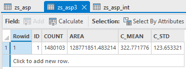
Ok, we have some results that have solid meaning. The average for the circular aspect values with standard deviation.

You can evaluate your circular mean by translating the value to the direction and color. Inspect your watershed for that color.

 

Why isn't the tool calculating min and max and the other statistics.
For one thing, min and max aren't meaninful statistics with circular data. But Majority and Minority might be...

Quick Google search uncovered an Esri community hint that converting to integer values could make a difference. 

It's really important to evaluate your results. Check back to the map.

 

These landscape characteristics can be used to compare watersheds, better understand watershed response to fire, runoff, stream power.

 

And that's it! You have successfully delineated a watershed and characterized the potential stream network and landscape characteristics within.