Open Source (read: FREE!) GIS

This lab was created by Alan Kasprak at Fort Lewis College

This lab will introduce you to working with airborne lidar data and alternatives to ArcGIS for visualizing, analyzing, and presenting those raster data and their derivative products.

The goals for this lab

1. Show you how to search for and download lidar data from a national repository.
2. Introduce you to CloudCompare, a free utility for turning lidar points into continuous rasters (and tons of other stuff, too) and show you how to load and visualize point cloud data, along with exporting those data to a continuous raster DEM.
3. Introduce you to QGIS, an alternative to ArcGIS, where you’ll gain familiarity with basic raster analysis and generating presentation-quality maps.

Part 1: Download Lidar Data from OpenTopography

Open Topography is an NSF sponsored facility based at the University of California San Diego’s Supercomputing Center. It is operated jointly with Arizona State University. They strive to make high resolution and valuable lidar data available to the public. Open Topography is a site that "facilitates community access to high-resolution, Earth science-oriented, topography data, and related tools and resources.”

This demonstration will show you how to create a digital elevation model from lidar point data. Did you know that lidar starts as points? A laser is shot from an airplane (typically) and bounces off the ground. The bounce location is mapped as a point and is attached to the elevation at that location. The elevation is calculated from the return time of the laser light (+/- the angle of the mean, and tilt pitch and yaw of the aircraft). The result is thousands or even millions of points with an associated elevation value. That is lidar point data.

To start, I recommend creating an account at OpenTopography. While an account isn’t necessary to download all of the data on OpenTopography, if you want to use any of the USGS 3DEP Data, it is - and that account needs to be associated with a .edu email address, so make sure to use your aggiemail email address.

To create an account, click My Open Topo in the header bar at the top of the page, and then click Create New Account at the bottom of the page that opens. Walk through the steps, remembering to use your aggiemail email address, and in a few minutes you should have an account. Remember your credentials, because you’ll need them to log in to OpenTopography!

Once you’ve got an account set up

• Go to opentopography.org and click Data - Find Data Map, which will take you to a map with lots of lidar datasets marked by dots.
• Zoom to an area of interest

For this lab, I’m going to leave the choice of locations up to you, but I’d like you to download two sets of lidar data: one for an area that’s relatively steep/rugged/high relief/mountainous, and one for an area that’s relatively flat/smooth/low-relief. Your challenge will be to make two sets of maps, both of which provide an interesting perspective on two very different places. I’d suggest working through everything using one dataset first, then coming back and repeating the process with your second location

• Click on an area of interest; remember that if you click a USGS 3DEP Dataset (the ones in green), you’ll need to be logged into your account to download the data.
• Click on the dataset name hyperlink.

This will take you to a page with information about the data, including spatial extent of the dataset, survey date, how many return points were collected, the point density and resulting raster resolution, the coordinate systems, and metadata files.

Most important is the coordinate system! I would recommend copying and pasting the coordinate systems into a word doc so you have the info for the LAS conversion tool that we’re going to use in a second.

• Click Point Cloud Data under the Download and Access Products header.

In the map area that comes up, click ‘Select a Region’ and then draw a sub-region to download. Keep it small! A mile square is plenty, and there is a limit to what you can readily download and process for an exercise like this! If you find that later on, the steps are going very slowly and things are crashing, come back and downsize your data request. Scroll down and you’ll be warned in Section 1 if you’ve chosen too many points.

• In Section 1, under “Choose Return Classification”, select only Ground
• In Section 2, choose to download point cloud data in ASCII format
• In Section 3, don’t have them generate a TIN. Nothing should be checked in Section 3.
• In Section 4, don’t have them generate Hillshades or Slope grids, we’ll do that ourselves later.
• Same with Sections 5A, 5B, and 6 – don’t check anything.

Give your job a title, short description, and provide your email address. Hit Submit, and when the job is done processing, you’ll get an email with a download link.

When your job is complete, download the various products by clicking on them in the email you receive. The ASCII file will be compressed into what’s called a ‘tarball’ archive. Note that this “.tar.gz” file is actually zipped twice. You can use 7Zip to extract these by right-clicking, going to 7-zip, and selecting Extract Files. Do this twice. The first extraction will get you a “__.tar” file (getting rid of the “.gz”), and then run the extraction again to get a regular folder with data in it.

Also download the metadata file for the job in the top right of the page, which contains the coordinate system info you will need later.

Part 2: Installing CloudCompare and QGIS

Both of these programs should be on the lab computers. However, what’s nice is that both of them are also completely free, and so what follows is a quick introduction to each, and instructions for installing them on your own home machine or laptop, if you’d like.

We’ll need two programs this week. The first, CloudCompare, will let us display our point cloud file and export that point cloud as a DEM. The second, QGIS, will let us run some raster processing steps on that DEM and make a map that will be submitted.

First, let’s get CloudCompare. Go to the home page, click Download, and then select the version that’s right for you. The Latest stable release is probably the best choice.

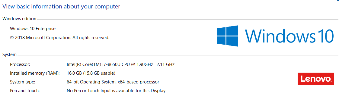
I’m assuming everyone is running Windows, so first you’ll need to check if your Windows version is 64 or 32 bit. You can check this by opening up File Explorer, right clicking on “This PC” - Properties and check what it says under “System”. I’ve got a 64 bit processor, so this is what mine looked like:

If you’re running 32 bit windows, a bit further down the page is a link to the 32 bit version of CloudCompare, which is no longer supported (the vast majority of computers are 64 bit these days) but the old 32 bit version should still work for this exercise. If you’re running MacOS, there’s an installer for that too, and one for Linux as well, if you happen to be that cool.

Once the download is complete, run the .exe installer, accept all the default options, and you’ll have a working version of CloudCompare soon. If it prompts you to restart your machine, go ahead and do that now.

Go to QGIS and go down to “Standalone Installers”, make sure you select the “Long Term Release – Most Stable” and select the 64-bit or 32-bit option, depending on which processor you have, just as above. Again, MacOS and Linux users, you can download what’s best for your system - unlike ArcGIS, QGIS will run on platforms other than Windows!

Part 3: Working with lidar data in CloudCompare

Open up CloudCompare. This software has a ton of features for (as the name implies) comparing point clouds to get at landscape difference over time, classifying point clouds into different landscape cover types, assessing point cloud precision and accuracy, and lots more. Today we’ll barely scratch the surface of what it can do.

Go to File - Open - select your .txt point cloud. You may have to choose “ASCII cloud” from the Format Type dialog in the bottom right.

A spreadsheet window will pop up with a snippet of your data. This is CloudCompare asking you what columns of the file correspond to what values (easting, northing, elevation, intensity of laser return, etc). The point cloud file you downloaded from OpenTopography has a lot of columns, so click and drag the window to expand it and have a look at all the columns (or use the bottom slider to pan over).

Go down to where it says “Skip Lines” and set that to 1, which tells CloudCompare that the first line of the ASCII point cloud is a header, and not actual data. Then use the drop-down menus over each column to set up the data import just like what’s shown below (first three columns are X, Y, Z, and ignore the others):

Hit Apply all; a window will come up asking if CloudCompare can simplify/shorten the X and Y coordinates to save memory. You can say Yes to All, we’ll get the coordinate precision back when we export data in a couple minutes.

It’ll take a minute for the cloud to load up. When it does, you’ll be looking top-down at the landscape as if you were in an airplane flying overhead. Now you can play around with the view a bit more. Use the left (main) mouse button to click, hold, and drag on the screen and you’ll notice you can move the point cloud around to get a better view. The mouse wheel will zoom in and out, and holding the right click button will let you move the whole point cloud around.

If you ever get really lost, you can always click the boxbox again to re-orient yourself.

You can change the colors of the background and points by going to Display **- ** Display Settings - Colors and Materials. You can easily export the current point cloud view by going to Display **- ** Render to File.

Okay, now let’s make a digital elevation model from our point cloud. This will essentially come down to connecting the dots to form a continuous surface – but in this case there are many, many dots. In the top menu bar of CloudCompare, click the checkerboard icon to generate a raster raster tiles

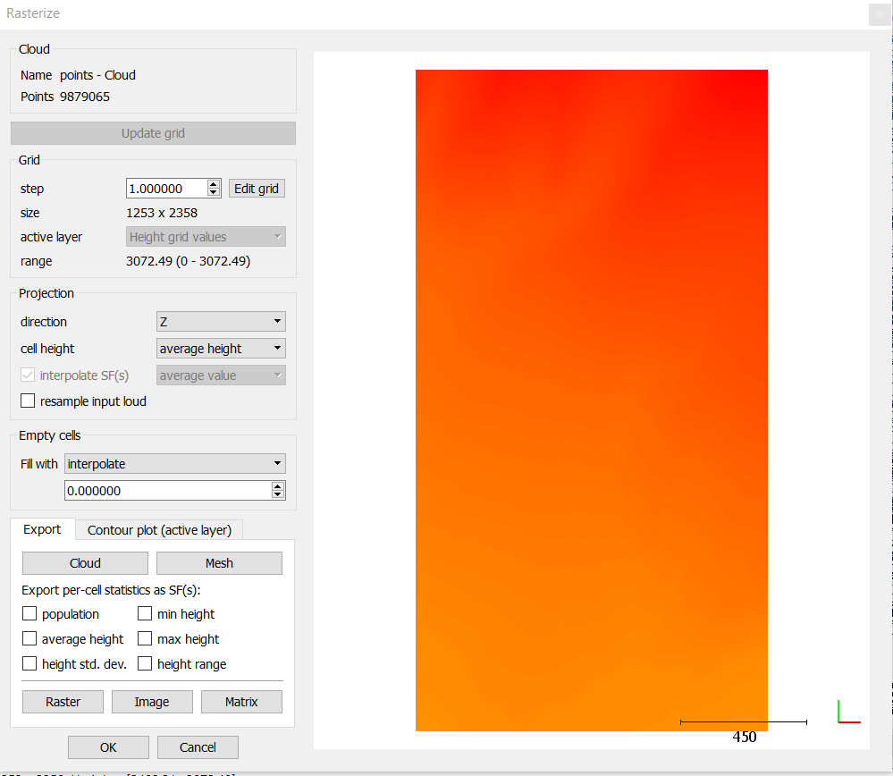
If it’s greyed out, click the name of your cloud in the table of contents to select it. When the Rasterize window opens, click Update Grid and a DEM should appear. Set the Direction to Z, Cell height to Average Height, Fill With to Interpolate, and leave everything else as it is. Your window options will look like this, although your DEM preview will surely look different. Make sure you hit ‘Update grid’ prior to exporting!

Click Raster to generate a DEM. In the dialog box that pops up, the only thing you should check is Export Heights. Give the DEM a filename and save it somewhere you’ll remember. Once it’s saved (which should only take a few seconds), you can exit CloudCompare.

Part 4: Working with lidar data in QGIS

Go ahead and open up QGIS. You’ll notice that the interface looks fairly similar to ArcMap, with a table of contents on the left hand side of the screen and a bigger mapping window on the right.

Now let’s open up and display the DEM we just created in CloudCompare. To do this, click the “Open Data Source Manager” button (the three squares with the plus sign all the way on the left of the top toolbar).

A menu will pop up displaying the many types of data that QGIS can load. Select Raster, and then locate the DEM you just generated. Hit Add and close the import window.

You might see an orange warning bar in the top of the map viewer letting you know that QGIS doesn’t know what projection the DEM is in, and as a result it’s assuming it’s in WGS 84.

Is that right? Recall the coordinate system of the lidar data you downloaded (you hopefully wrote these down earlier in the lab, or you can check the metadata file you downloaded).

If WGS 84 isn’t the right coordinate system (or even if you didn’t get an error, it’s good to double check anyway!), you can change it by right clicking on the DEM in the table of contents, selecting ‘Properties’, and then in the “Source” tab, you can select the appropriate coordinate system from an extensive list. You can use the drop-down menu to select the project CRS as well, assuming you chose the right one a second ago. Highlight the appropriate coordinate system, hit OK, and then hit Apply in the Properties window. Back in the map window, you may have to right click on your DEM and Zoom to Layer to get it back in view.

This is also a good time to set the Project’s CRS. Go to Project - Properties and select the same CRS that you just applied to the DEM. This will ensure that any layers you subsequently generate will be in the correct CRS. Save your project by clicking Project - Save As… and giving it a filename.

Now go to Processing - Toolbox, which will open up a very ArcGIS-like menu on the right hand side of the screen that should look familiar, with many tools that operate on vector and raster data. We’re going to do a few processing steps with our DEM.

• Hillshade: Raster terrain analysis - Hillshade; use your DEM as the elevation layer and accept the defaults. Note that QGIS will save these outputs to temporary files, but you can and should specify an actual, permanent output .tif file. You may receive a warning that the coordinate system was undefined, but as long as you defined your DEM’s coordinate system when you imported it, QGIS will default to the correct one for the hillshade.
• Slope: Raster terrain analysis - Slope; use your DEM as the input.
• Ruggedness (one of many ways to estimate roughness): Raster terrain analysis - ruggedness index; use your DEM as the input.
• Aspect: Raster terrain analysis - aspect; use your DEM as the input.
• Contour: you’ll want to search for this one in the Processing Toolbox (it’s under GDAL toolset at the bottom of the list). Choose an appropriate contour interval for your data.

What to Submit

For this lab, you’ll submit two maps, both on your website:

Make these your best possible maps of the elevation data and associated information that you can generate using QGIS. Present any combination of the DEM, hillshade, aspect, ruggedness, slope, or contour data you’d like. Include the standard components of a good map (scale bar, north arrow, etc.) You can combine these into one single map showing both of the lidar locations you used, or you can make two separate layouts. If you’d like to only map a smaller portion of your data’s full extent, that’s completely fine by me.

If you’d like to do more spatial analyses in QGIS on top of what you’ve already done, you can present those results as well. Basically, show me the best map you can make in an open-source and free GIS. Don’t cheat yourself this week and just try to rush through the output! Make the best layout you can, go through the options, and learn QGIS a bit. Don’t be afraid to break things (just remember to save your map often). We’ll use QGIS next week too, so I want you to get to know the software a bit.

You are rapidly becoming independent and high-level GIS analysts. That said, I’m not going to walk you through a layout in QGIS step-by-step this week. I want you to independently figure things out, much like if you were working as a GIS professional and needed to quickly learn some new software.

Of course, here are a few helpful hints…

• Right clicking on a layer in the table of contents will bring up its properties. From there, you can set color ramps, transparency, line thickness, and lots more.
• You can order layers by dragging them just as you would in ArcGIS. Remove a layer with right click - Remove Layer
• Get your map displayed just the way you want in your main QGIS window, then go to Project -> Layout Manager to create a new page layout. Name it whatever you’d like.
• In the layout, click “Add Item - Add Map” and use your mouse to draw a rectangle where the map should go. This is pretty similar to ArcGIS Pro. It will be immediately populated with whatever map was displayed in the main QGIS window.
• Other items (legend, scale bar, etc.) can be added in the same way (Add Item - Choose what you want) and drawing a rectangle where it should go. The properties and appearance of any item can be changed by selecting that item and then choosing the Item Properties tab
• Continuous color ramp legends can be a bit tricky, so see here for some tips on adding a 'color ramp' rectangle on adding a ‘color ramp’ rectangle to get around this.

The QGIS documentation page on layouts has a TON of information on how to generate, populate, and export layouts as PDFs, TIFs, JPGs, and anything else you can think of. So if you need help, start there.