Introduction

In this part of the lab we will explore ArcGIS Pro’s Suitability Modeler, a tool that streamlines the process of combining and classifying raster layers. Unlike manual methods, the Suitability Modeler allows you to adjust weights in real-time using a power function to instantly see how these changes affect your results. This exercise builds on the previous work with the Spotted Owl and provides a brief demonstration of setting up a simple suitability model to highlight its capabilities.

The demonstration focuses on preparing 4 different data layers for the model - transforming their original values into normalized suitability rankings.
We will cover the transformation of:

• Continuous data
• Categorical data
• Classified continuous data

 

Download and open this ArcGIS Pro Package to get started.

... and before anything else can happen:

The Ever-Critical Data Inspection

First inspect the layers in the contents pane. 

The top layers are a stream polyline layer [streams_major_aoi] and a distance raster [dist2stream] calculated from the polylines.

The distance layer was calculated using the Distance Accumulation tool which generates a raster in which each cell value represents the distance (m) to the nearest feature.

The range of values indicates that there are locations in the raster that are over 14 km from the nearest major stream polyline.

You won't need the Stream polyline layer. It was just provided for visual context.

 

Turn off the visibility of the Streams and Distance to Streams layers.

 

The Slope layer [slope_d] indicates that the value units are degrees. 
Does it make sense, then, that the max slope value is around 84 for an area like this?

Turn off the visibility of the Slope layer.

 

Open the attribute table for the Landcover- existing vegetation type layer [landfire_evt].

We will be using the EVT_PHYS field for our classification. This field contains the most general description of the landcover types and will be easiest to classify.

Close the table. Turn off the visibility of the Landcover layer.

 

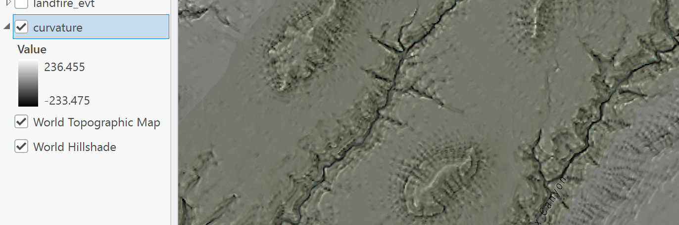
Inspect the range of values for the Curvature layer. What do these mean or represent, exactly? 

If you aren't familiar with Curvature - in the most general way it is the slope of the slope and can describe whether a cell is convex or concave, whether "flow" would accumulate or disperse across its surface. 

It helps to inspect curvature over a hillshade or terrain map.

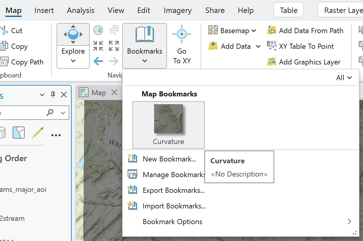
I've bookmarked a scale that works well for inspecting positive and negative curvature values on the landscape. 

Under the Map ribbon, Navigate panel, click the Bookmarks dropdown and click on Curvature. The map will zoom in to a preset area of interest.

 

Notice how the dark and light cells align with the valley bottoms and ridges, respectively. Make mental note that positive curvature values represent convexity and negative curvature values represent concavity. 

 

Now you know the data you'll be working with.

 

Suitability Model

Create the Model

Analysis tab > Workflows pane > Suitability Modeler - Click it.

"New Suitability Model" layer is added to the Contents pane (it's empty).
The Suitability Modeler tool opens to the Settings section.

Model Name can be changed if you want. I'll be referring to ours as the "Owl Model."

I'm leaving the input settings for Model input type, Suitability scale, and Weight by as they are.

Name the output suitability Raster Layer: I named it "owl_model"

 

Add the Model Criteria

Click over to the Suitability tab.

 

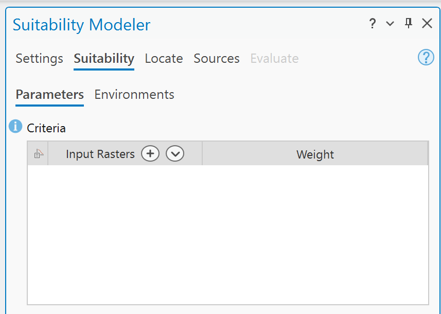
This is where you will add the criteria for our model.

Criteria for the Spotted Owl habitat model:

• Distance to streams - less is better
• Slope should be steep
• Curvature should be on the extreme side of concave and convex
• Landcover should be 'wooded'

 

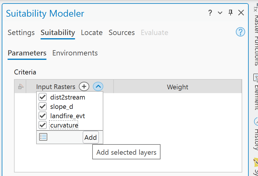
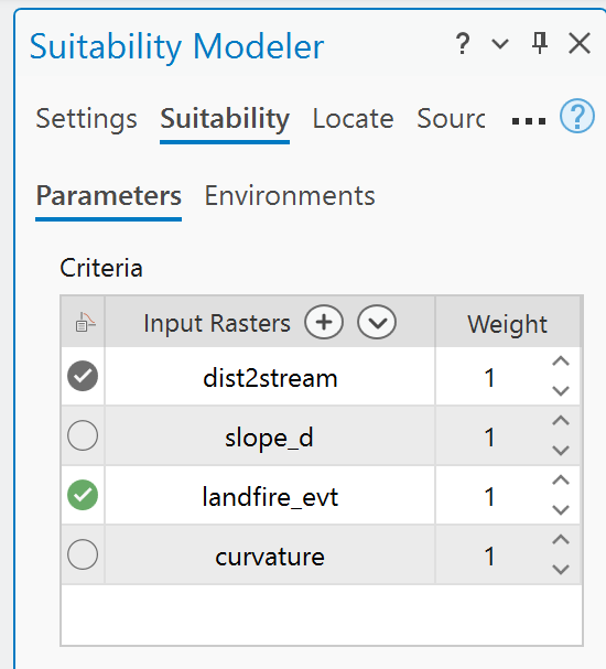
Click Add.

Four input rasters should be added to the list, and the contents pane will also reflect the addition of these 4 rasters to the model.

 

 

Adjusting Continuous Data

The first layer we will transform is the distance to streams raster.

Click the radio button in the Suitability Modeler - Suitability tab - Criteria window.

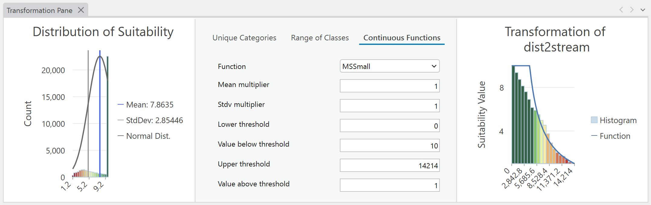
This activates the Transformation pane that shows the distributions of the values in the raster (on the right) and the distribution of the accumulated suitability values on the left. We only have the one criteria in the model so far, so the suitability distribution isn't telling us much. 

 

 

Two new layers were added to the group in the Contents pane: owl_model and Transformed dist2stream. 

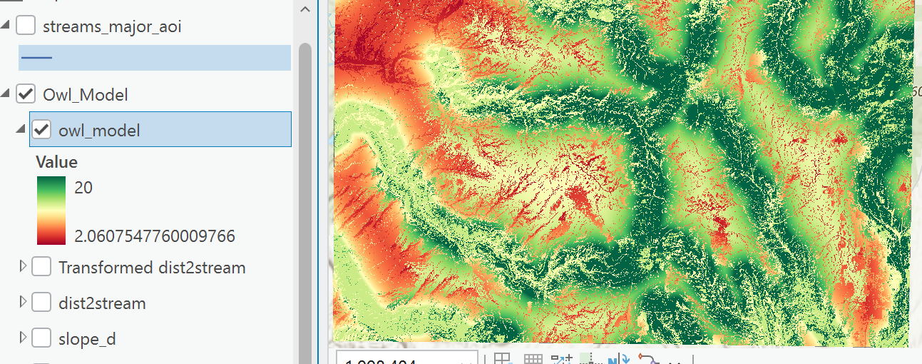
Notice the range of values for the transformed dist2stream layer is 1-10. This is the range of suitability values we assigned in the Modeler settings. 

 

 

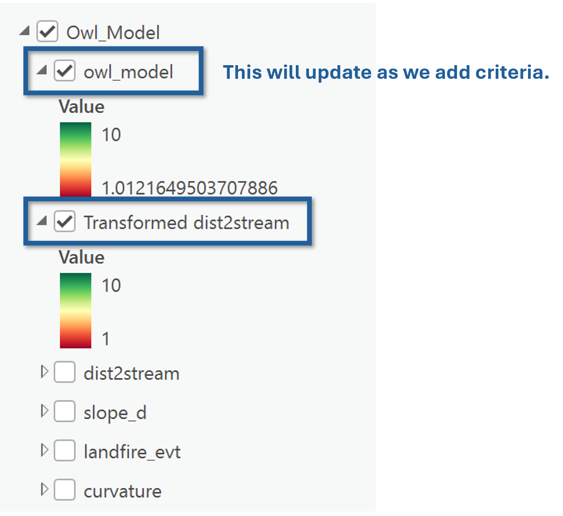
Zoom to Layer on Transformed dist2stream so you can see the full extent of the transformed distance raster. 

10 is the most suitable, 1 is the least suitable.

The green areas (10) are the areas closest to streams, so this looks correct.

But we don't take default settings at face value. Right?

No, we don't.

 

Let's deep dive into the Transformation pane.

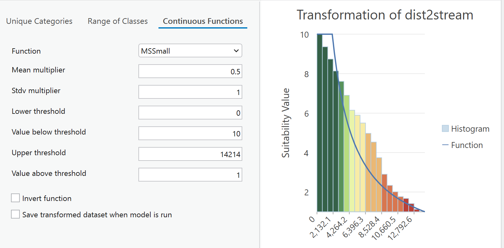
The histogram shows the distribution of values and is colored according to the function applied. 

 

 

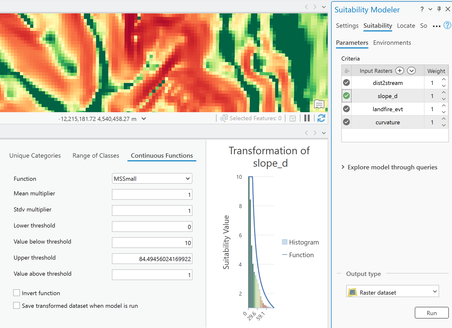
The default function in MSSmall, which stands for Mean-Standard Deviation Small.

You can see the Functions in the middle section of the transformation pane - in this case we are looking at the options for Continuous Data Functions.

 

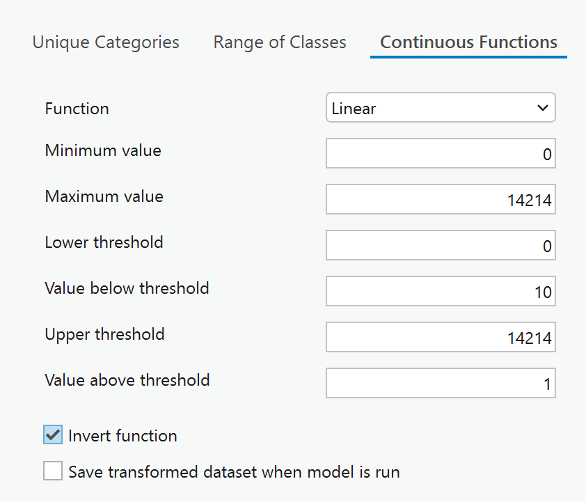
Experiment by changing the Function to Linear:

 

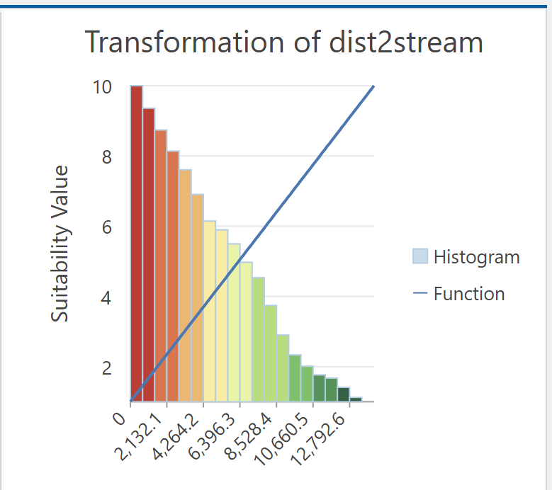
Notice that the smaller distance values have been changed to red - meaning they are being considered unsuitable, which is incorrect for our model. 

No big deal. We can Invert this function by clicking the Invert function button

 

 

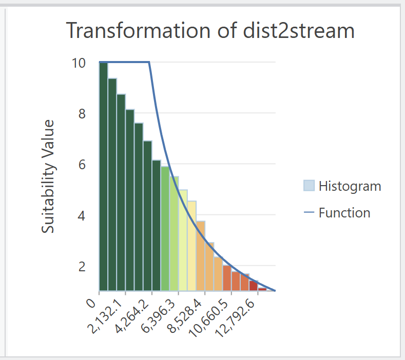
Look at the symbology on the map. The main difference is the graduation of green. This is much more gradual and the suitability graduates as we move away from the stream.

MSSmall function considers all distances within around 5000 meters to be highly suitable (10) and then suitability values drop away quickly.

We can change the threshold distance at which that drop off starts to occur by using the Mean Multiplier setting.

For example, if we wanted that distance to be half of that 5000 m - say more like 2500 meters, we could multiply the mean by 0.5.

 

 

Adjusting Categorical Data

 

Now, let's add a second raster layer to our model.

The next data we will transform to the normalized 1-10 scale is the landcover data.

Recall that this is a raster layer where the cell values represent unique vegetation or landcover types. These values can't be treated as continuous. 

 

In the suitability modeler Criteria panel, click on landfire_evt:

 

 

Updates are made. Notice the range of values for the "owl_model" in the contents pane has expanded to a max of 20. That's because we have added landcover suitability to stream ditance suitability.

Notice that the transformation pane has updated the distribution plots and the middle section has changed automatically to Range of Classes.

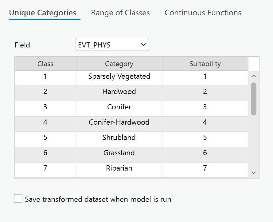
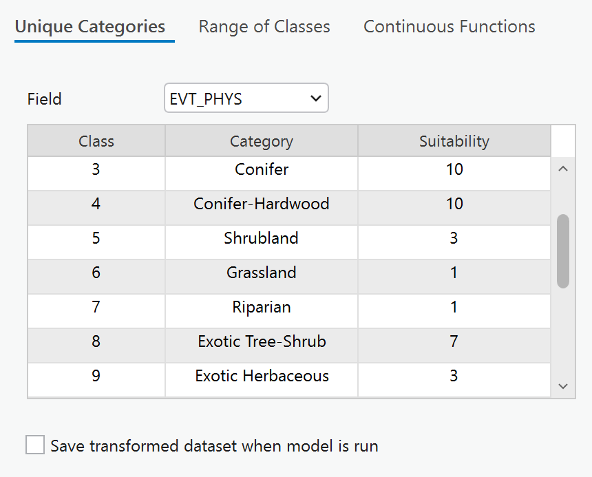
We are going to instead work with Unique Values. So switch to the Unique Categories tab.

And the Field we want to transform is EVT_PHYS (remember? because it contains a general description instead of the hyper-detailed descriptions in some of the other fields).

You should see this:

 

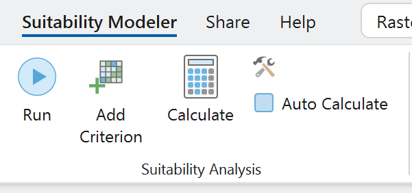
Before setting suitability values for the landcover types, turn off the Auto Calculate function or you'll be waiting around for temporary adjustments every time you assign a value.

On the main ribbon - Suitability Modeler Tab > Suitability Analysis panel > uncheck the AutoCalculate box. 

 

 

The categories that are most suitable (10) are:

• Hardwood
• Conifer
• Conifer-Hardwood

Categories that are moderately suitable (7) are:

• Exotic Tree-Shrub

Categories that are less suitable (3) are:

• Sparsely Vegetated
• Shrubland
• Exotic Herbaceous

Categories considered unsuitable (1) are:

• Grassland
• Riparian
• Open Water
• Barren
• Quarries Strip Mines - Gravel
• Developed Low, Medium, and Roads
• Agriculture

Go through and assign these suitability values to each of the landcover categories.

Here's a partial look at the changes:

 

 

Now go up to the Suitability Modeler tool ribbon and click Calculate and turn the Auto Calculate back on.

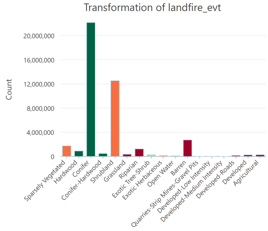
Check out the results in the map. 

 

 

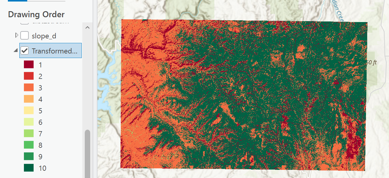
The symbolized frequency distribution looks something like this:

 

Turn on the visibility of the owl_model and see what the updated suitability model for our owls looks like. The dark green areas map cells that are both suitable landcover and suitable distance to streams.

 

 

Saving your Suitability Model

Saving the model is Different than saving the project. 

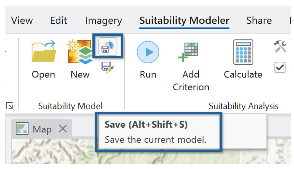
You can save your Modeling progress using the Save icon in the Suitability Modeler tab > Suitability Model panel.

 

Once it is saved, you can close ArcGIS Pro and come back to this model later, picking up where you left off.

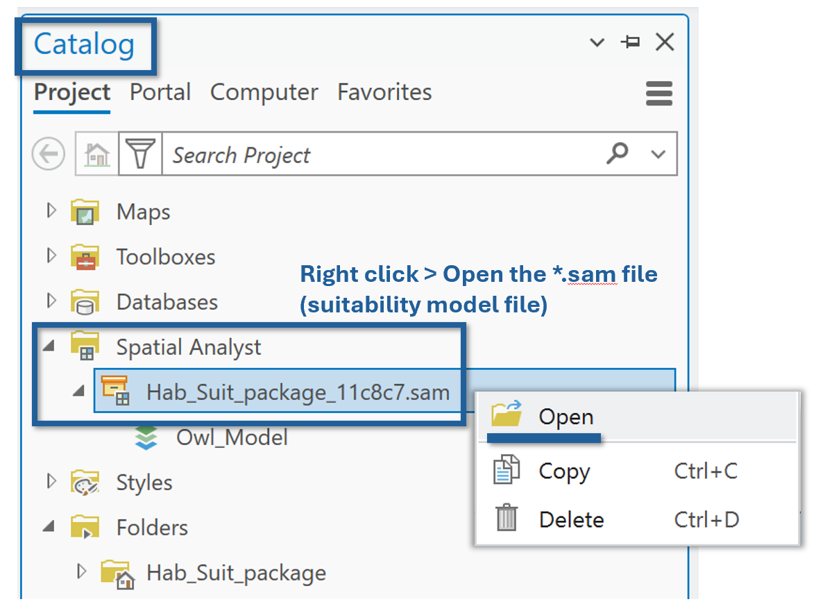
If you close the Suitability Model and need/want to reopen it, you can find it in the Catalog > Spatial Analysis tab > find your *.sam file > Right Click to open.

 

Adjusting classified continuous data

 

We are going to classify the Curvature layer to impose strict limits on the suitability of convex and concave surfaces.

Turn on the Curvature layer in the Criteria window.

 

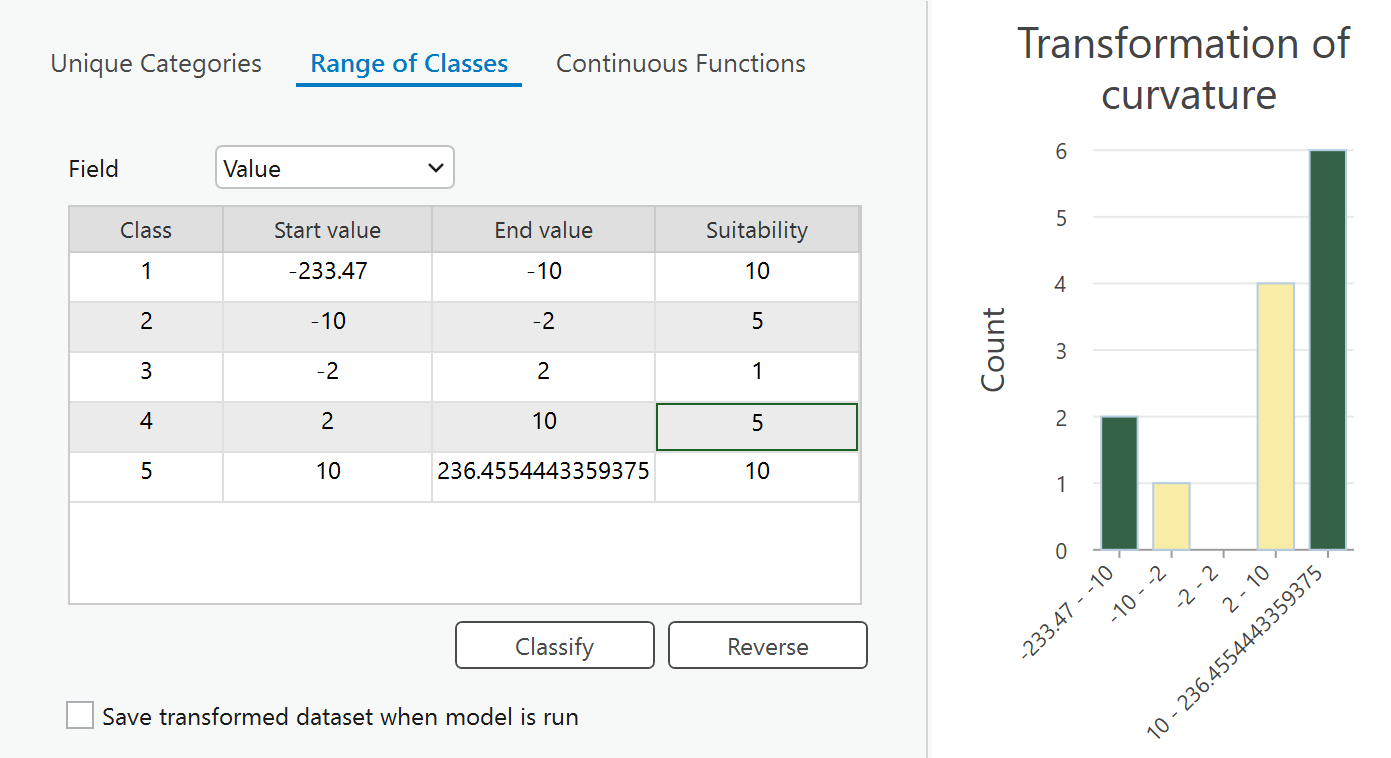
In the Transformation window, set the type to Range of Classes and use the Classify button to adjust the class break values.

Create 5 classes with the following values:

• minimum curvature - -10.0  =  suitability (10)
• -10 - -2.0  =  suitability (5)
• -2.0 - 2.0  =  unsuitable (1)
• 2.0 - 10.0  =  suitability (5)
• 10.0 - maximum curvature  =  suitability (10)
  
  

Inspect the suitability of curvature on the map - compare to the original curvature to ensure that both ridges and 'troughs' are now mapped as suitable (value 10).

 

 

Notice that the owl_model now has a max value of 30, meaning we have incorporated 3 of our input criteria and that some locations are suitable for all 3 input layers.

 

Transforming data using the Power Function

untz untz untz

 

Activate the Slope layer in the Criteria panel.

Notice the transformation window updates automatically to Continuous Functions.

 

Switch the Function to Power.

 

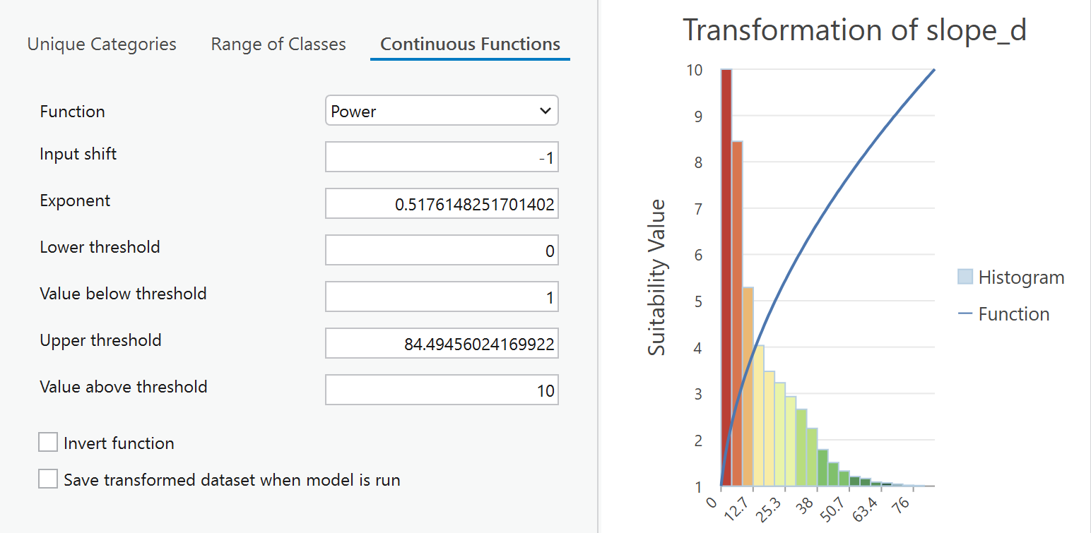
High slopes are green and assigned values of 10 (the function line).

If we want to bend the curve of the function line more, we can change the Exponent value to 0.2 (experiment!). But this adjusts lower slopes into the highly suitable range, and we want to keep the most suitable slopes to reflect the steepest slopes. (So return the exponant to 0.5). 

 

Now our owl_model has a max value of 37, which means there aren't any perfectly suitable locations, but some that are highly suitable.

 

from: https://beautifulhighschoolmath.blogspot.com/2015/09/precalculus-parent-functions.html

 

 

Weighting the Criteria

Weighting assigns importance to the input layers.

 

Landcover and curvature are most important to defining suitable habitat (for the purposes of this exercise).

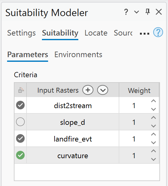
Set weights in the criteria window like this:

Dist2stream  =  1
slope_d  =  1
landfire_evt  =  2
curvature  =  3

 

If you have turned off auto-calculate, remember to turn it back on and use the Calculate button to refresh the model calculation.

 

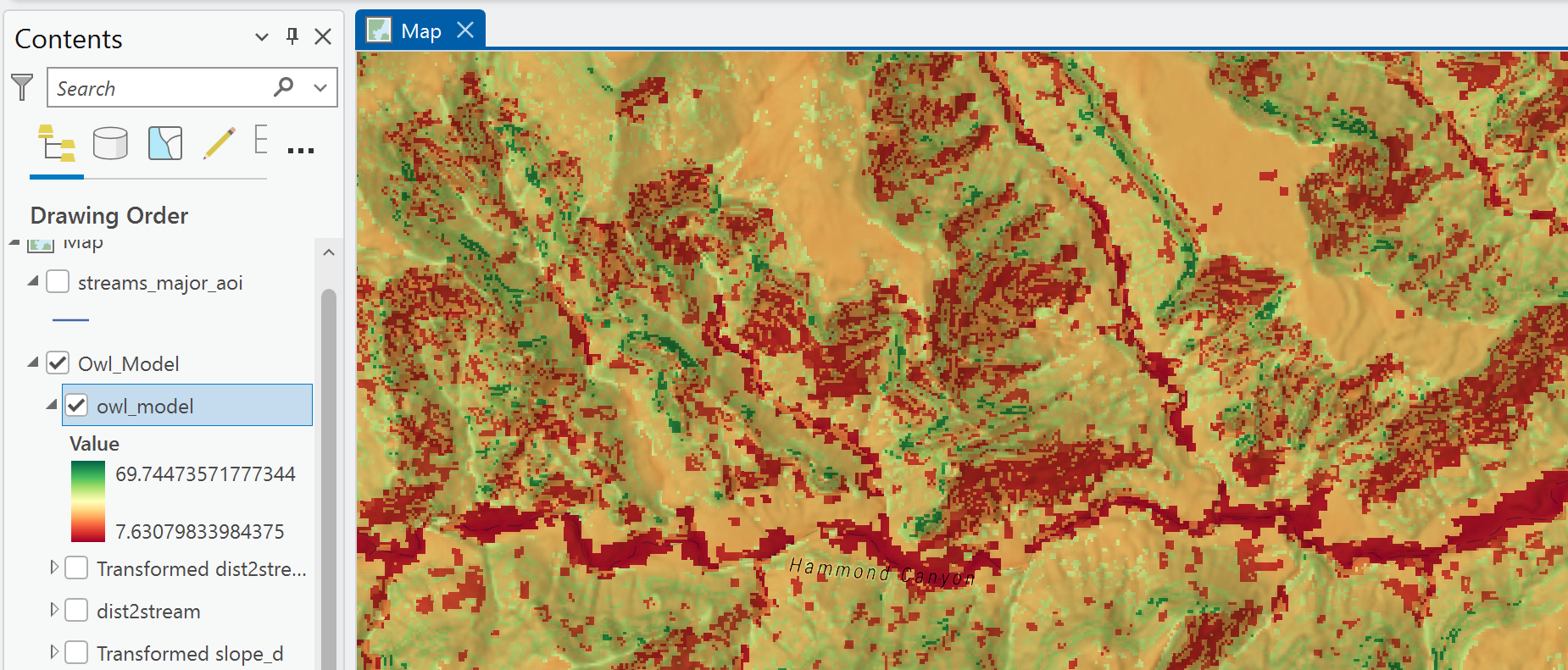
Notice the range of owl_model values has blown up - showing ~70 as a max value. This is because we multiplied our curvature suitability values by 3 and landcover values by 2 before adding them to the slope and stream distance layers.

In the image, I used the Multiply Layer Blend option to display the owl_model layer over a terrain basemap. 

 

Ready for the last step?

 

 

Automate Location of the most suitable sites

 

In the Suitability Modeler Panel, switch to the Locate tab.

 

Set up the inputs to identify 3 total areas of at least 10 acres each:

 

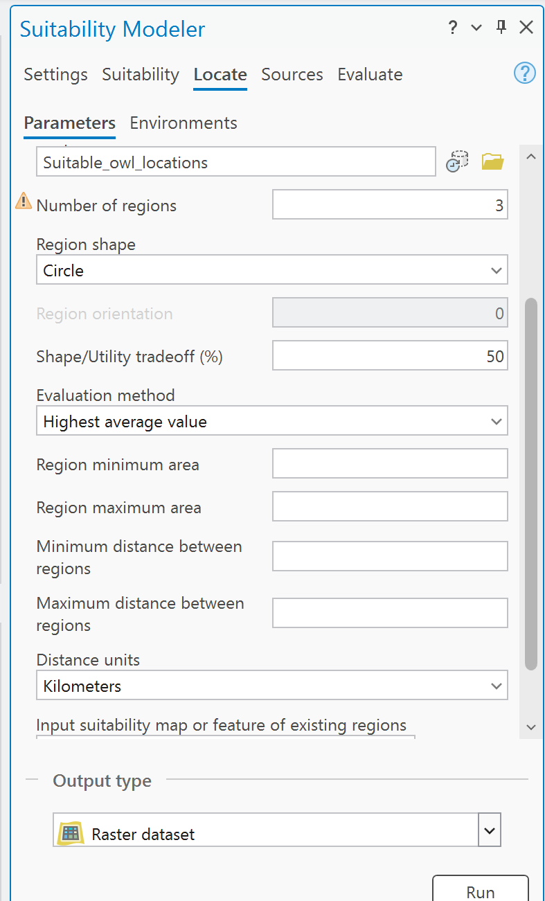
Run Locate.

Watch the task bar work through the steps. It is fascinating. 

 

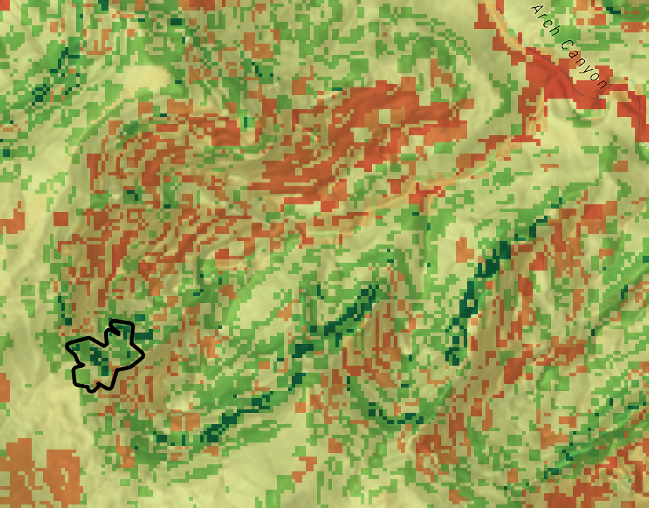
The output is a RASTER.
To visualize the locations, convert raster to polygon and control the symbology.

 

The Locate tool maximizes the balance between suitability values and area to produce the number of final areas we designate in the tool. 

 

 

And that's it.
Obviously you could and should experiment with applying different functions to the input criteria and apply functions that suit your needs.