Habitat Analysis:
Northern Gannet Nesting Sites

Photo Credit: Ray Harrington

The Basics:

The Audubon Seabird Restoration Program is looking to expand the nesting colony sites for the Northern Gannet along the northern Maine coastline.

Northern Gannet are cliff dwelling coastal sea birds, the largest of the North Atlantic.

For the purposes of this analysis, use the following generalized habitat preferences for Northern Gannet nesting colonies:

1. Areas with a slope greater than or equal to 80%
2. Must be on the coast (see details below)
3. Must be 300 meters away from a public roadway
4. Nesting site must be at least 1 hectare in size

After completing the analysis, evaluate your results and present a map that clearly displays the resulting habitat
areas.

Photo Credit: Stephen Lytle

The Data:

There are only three datasets you will need to complete this exercise:

• MaineDOT_Public_Roads: Public roads polyline (https://maine.hub.arcgis.com)
• ME_10mDEM: 10 m DEM (USGS National Map)
• Maine_Boundaries_County_Lines: Polyline mapping county boundaries (https://maine.hub.arcgis.com/)

Note: You will notice that the dataset extents are not the same between the line maps and the DEM. The area of interest to the Audubon Program is constrained by the DEM’s extent.

Set Display Coordinate System:

Change the display of your map to match the public roads layer. We haven’t worked with State Plane coordinate systems, yet. They are small projections focused on portions of each state, making them somewhat similar to UTM in performance, but available just for the US.

Approaching the analysis

Think through the general habitat rules:

1. Steep slope (greater than 80%)
2. Near the coast
3. Away from roads
4. At least 1 hectare in size

• You have elevation data from which you can calculate slope.
• You have county boundaries that contain a designation for coastline (wow, that’s helpful!).
• And you have a road dataset.

Does the order in which you attack these rules affect the analysis? No.

Challenge yourself to do this without instructions as much as possible.
I provide a little instruction on reclassifying the slope data. But other than that, you have all the skills to complete this analysis on your own.

Criteria #1: Areas Must have slopes > 80%

Slope Analysis:

Map areas of slope that are 80% or steeper.

Steps in brief:

1. Calculate slope in percent rise
2. Reclassify to isolate steep cells
3. Convert the results to polygons

Steps in detail:

1. Run the Slope tool
   1. Use percent rise as your units.
   2. Use a geodesic method
      
      Remember:

      Use smart naming conventions: "DEMname_slp"
      
      Raster file names have a 13 character limit.
      
      Slope can be calculated in degrees or percent rise. 80% and 80 degrees are very different!
       
2. Evaluate your results
   
   1. Check the contents pane.
   2. What is the range of values for the new slope layer?
   3. Remember 100% slope is a 45 degree slope.
   4. Do your results make sense?
3. Reclassify the slope layer using the ‘reclassify’ tool

The reclassify too can be tricky to use but worth taking the time to figure out. It is one of the important/commonly used tools you should master this semester.

 

Reclassifying a raster changes the cell values.

Example:

You want to isolate elevations above the tree line.
You can reclassify an elevation model. 
Create two classes, one representing elevations greater than your treeline elevation, and one representing elevations lower than the tree line elevation. 
Assign a new value of "1" to the class of elevations above treeline and "0" to the class below the treeline elevation. 
The output is a new raster containing only 2 values: 1 and 0
Converting the cells with a value of 1 to polygons gives you a map of the areas above treeline on your elevation model.

 

For this analysis, we don’t need the full range of slope values. We only want to know where the steep cells are. 

Thinking ahead… it will be easier to work with these areas if we convert the steep cells to polygon. 
We eventually want to convert the mapped steep areas to polygons so we can use tools like ‘select by location’ or ‘buffer’ and 'intersect' to choose the steep areas that fit the rules. And for the last criteria about a minimum area, calculate geometry can be used on polygons to measure the resulting areas.

Time Saver:
We could make you go through the exercise twice, once to see the reclassify output with new values of 0 and 1 and how converting that to polygon creates a solid block of millions of polygons that are almost impossible to work with… OR we can save you that step and save you time, but the cost is that you have to read this long explanation. 

 

You will use the reclassify tool to assign new values to the areas that are > 80% slope. The tool is called “reclassify” because you classify the data (break it up into 2 classes: < 80% and > 80% in this case) and then assign NEW values to the cells in those classes. Cells with slope values less than 80% will be given a new value of NODATA and cells > 80% will be given a new value of 1. Those are the "keeper" cells.

NODATA means that instead of a binary output with values in every cell in the raster, the not-steep cells will ‘go away’. The output raster will only have data where the slope is appropriately steep.

1. Search for the Reclassify (Spatial Analyst) tool
2. Input the slope raster you calculated
3. Make sure the Reclass field is set to VALUE
   1. The Value field in the attribute table is where the slope values are stored…
4. Create two classes
   1. Click where it says Classify below the list of values  
      
      
      
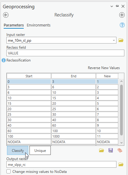
      1. Set the number of classes to 2
      2. Double-click in the cells to edit and adjust the values
      3. I named my output ME_slope_rc for ‘Maine slope reclass’
      4. Run

P.S. ArcGIS has a glitch with some of the classification methods. Sometimes the number of classes will be grayed out and unchangable. If you change the classification method to something different, it typically frees up the number of classes drop down.

Reclassify tool setup

Evaluate your results.

If you don’t see something similar to these results in your Contents pane, you may have goofed it up somehow. You should have a new reclassified slope layer with one value and one value only.

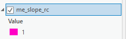
If you have more than the value in your reclassify results, run reclassify again on this new reclassified output. Change the "stray" values to new suitable values.

For example, if you have a stray value of 83, you would reclassify it to "1." 
A stray value of 14.5 would be reclassified to "NODATA." 
Reclassify "1" to "1."

 

 

• Turn off the visibility of all layers including the basemap so the screen is white.
• Change the color of the reclass slope layer to something vibrant.
• Right click the reclassified layer in Contents and ‘Zoom to Layer’
• Still don’t see anything? Zoom in…

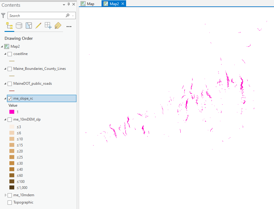
Luckily there are some steep slope areas to work with. Nice.

You can turn on a basemap again. Evaluate the locations against the basemap.

3. Convert the Rasters to Polygon

Why?

Because you need to select the steep areas that are near the coastline. Raster cells can’t be selected the same way features can. So, turn the raster cells into polygons. This will also aggregate proximate steep cells into adjoining areas for easy area calculations.

1. Open the tool “Raster to Polygon”
   1. Input is the reclassified raster (the one with only 1 value).
   2. Field should be set to VALUE (why? Because that is the cell value for a raster. That field is the one that will determine the polygons.)
   3. Yes, simplify polygons
   4. Don’t Create multipart features
   5. Run and evaluate your results.
      1. How? Turn off the other layers and zoom in. Do the polygon areas roughly match the steep slope cells? They should!

Example of the Raster to Polygon tool setup
Don't worry if the layer names are different.

You now have steep areas mapped as polygons. 

Criteria #2: Steep Areas Must be Within 100 Meters of the Coast

Start with the county boundaries vector data to find a proxy for the coastline.

Isolate the Coastlines

1. The County Boundaries dataset has an attribute field called Type.
2. Select by attribute to isolate all the polylines of Type "Coastline"
3. Export to new shapefile.

You now have a coastlines file you can use ensure your habitat areas are ‘near the coast’ (within 100 meters).

 

Map steep areas near coastlines

In brief:

1. Select steep polygons within 100 m of the coast polyline.
2. Save the selected steep coastal polygons as a new shapefile.

Rules #1 and #2 in the bag.

 

Criteria #3: Habitat Areas Must be More Than 300 m From Nearest Public Road

 

How are you going to do this?

 

 

I’ll wait.

…

Ok, here are some options I thought up:

1. Use Select by Location to select the steep polygons within 300 m of road lines
   1. “Switch” the selection to highlight the opposite (switch selection button found in the attribute table)
   2. Export the features
2. Use Select by Location to select the steep polygonswithin 300 m of road lines
   1. Delete the selected features

Select by Location has many selection methods. If you go this route, you need to decide if you will select steep areas that are completely outside the 300 meter zone around roads, or whether it is reasonable to select steep areas that are only partially within 300 meters of a road. OR you could use the Buffer and Clip method to cut the steep areas at 300 meters and delete polygons from within the 300 meter area.

Be aware of the impact this choice could make on your results. There isn't a "right" answer! There are processes that make sense for your data and your questions. Understanding when you need to make subjective decisions about your process defines intelligent GIS work.

1. Create a 300 meterbuffer on the road polylines
   1. “Erase” (this is a tool that does the opposite of “Clip” tool)
   2. Run "Union" which will combine the road buffer and the steep coastal polygons.
      1. Then select the polygons within the original buffer and delete.

Buffering and Erasing probably makes the most sense. 

Before you buffer all those roads, consider selecting roads that intersect the DEM area and removing the rest.

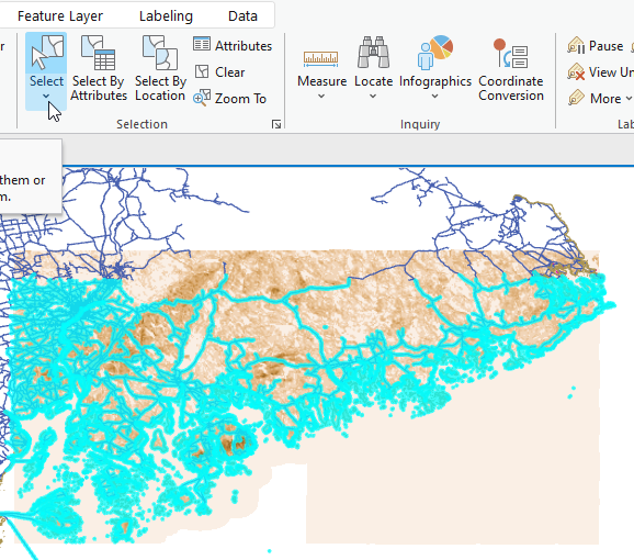
I loosely drew a rectangle over the DEM to select roads in the area of interest. No need to wait and wait for the processing buffering of all the line segments.

Evaluate your results.

Criteria #4: Nesting Site Must be at Least 1 Hectare

In brief:

1. Calculate the area of the remaining nesting locations.
2. Sort and select those that are at least 1 hectare.
3. Export the nesting sites > 1 ha to a new shapefile of your final sites.

Here is an example map showing the 4 resulting areas from my analysis. It is possible your results are different, and hopefully you identified some of the steps that might impact our results.

 

But hold on.

Did you have final areas that were greater than 1 hectare?

Sort the areas and select the biggest polygons. Zoom in and take a look at them.

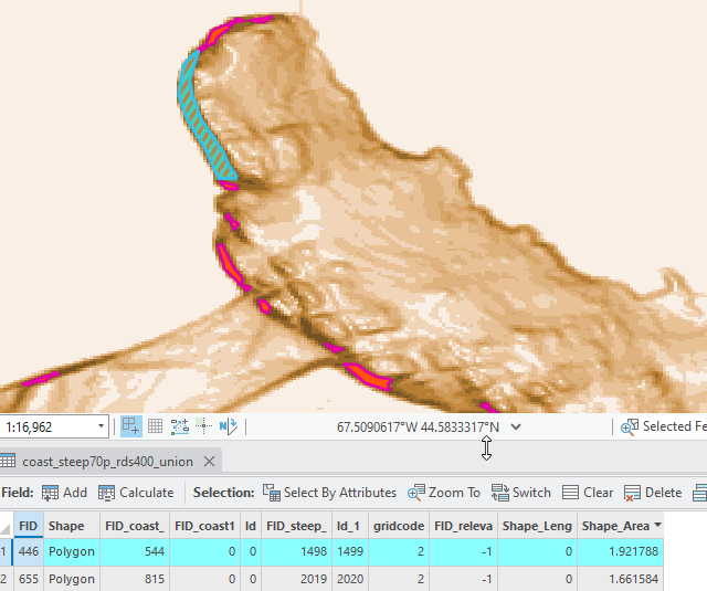
Again, the results may be different than yours, but look at the polygon sizes and proximity.
In this example it looks like there are very similar steep areas that are close by, but not connected. If these were connected, the resulting area would be bigger and there may be more potential habitat areason which to focus efforts.  

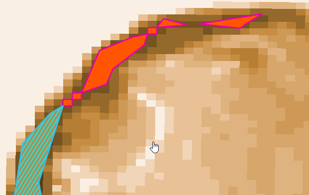
When we ran Raster to Polygon, we used the setting to simplify polygons. I'm not sure if the results would look different if we hadn't simplified. But this choice definitely impacted our results.

Question: What best suits our analysis goals? Is it reasonable to combine these polygons and treat the areas in the example (above) as one feature? Or should the polygons be kept separate?

In this case, I believe the processing tools and rigid threshold values (100 meters, 300 meters, 80%) justify a fuzzier definition of the final locations.

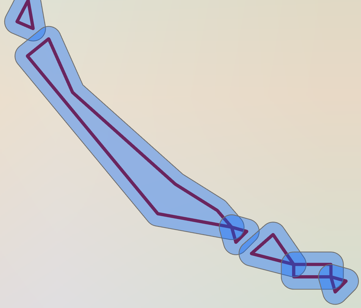
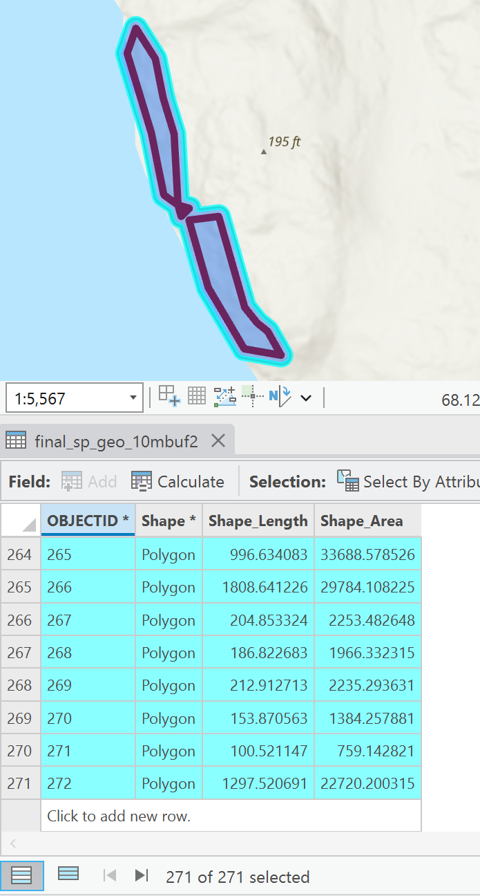
What could you do with this data to connect areas, like in the image above, that are very close but currently separate features?

My thought was to buffer the final polygons. 
Not a big buffer, maybe 10 meters? Use the measure tool to evaluate how a 10 meter buffer would change this data. 

Run a 10 meter buffer on your final areas:

 

In the pairwise buffer tool is the option to dissolve all features or not to dissolve...
Not dissolving results in individual buffers for each disjointed polygons. 

If you run the tool this way, you will want to run a secondary tool to Intersect or Dissolve overlapping features.

 

If you choose to Dissolve All features, you will end up with one big polygon (one record in the attribute table) representing multiple disconnected features.  

If you run the tool this way, you can "Explode" the features apart. 

Here's how:

Select the record in the attribute table.
Then in the Edit tab, find the Tools section and expand the window to see all:

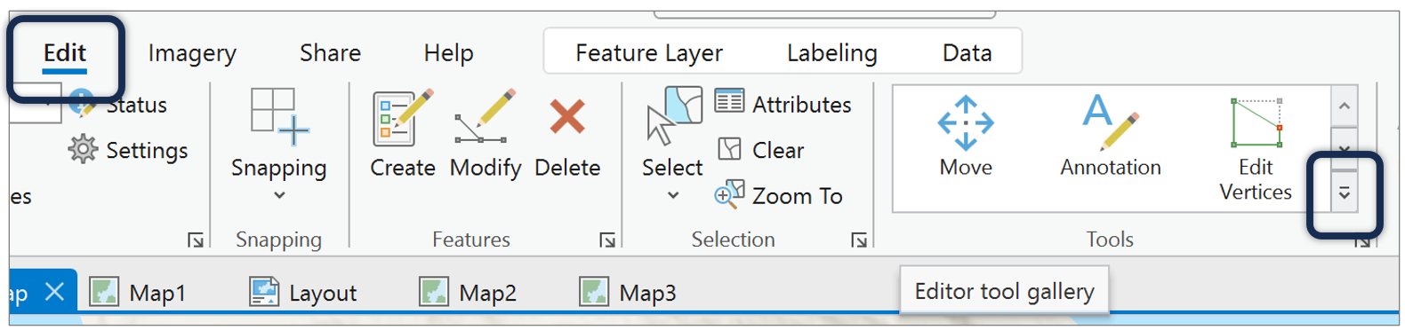
Find the Explode tool:

This is an Edit that you are making to the results. Remember to Save the edit when complete.

After exploding, view the attribute table. You should see many records, one for each new feature.

Remember, your results may vary!

Recalculate the geometry because the areas have changed and the area calculations don't automatically update.
Sort.
Highlight the biggest few polygons.
Zoom in and inspect. 

Do the buffered areas look reasonable over a hillshade or the slope layer?
Overlay your final results over the roads, coastline, and slope layers to verify.
Use Explore tool to sample the slopes within your final areas.

Finally, do you have areas greater than 1 hectare?
How Many?

I ended up with 23 (one was 0.99 hectares). More important than matching my results is understanding the decisions you made along the way that would impact your results. This is meant to drive home the point that the precision and accuracy of GIS results are strongly correlated with experience and level of critical thinking done by the analyst. 

Make a map of your top three largest areas and report each area in hectares.

Deliverable:

One document.

• Formal map focusing on 3 of the largest final sites
  • Exported to PDF, TIF or PNG
  • Not a screenshot
• Basemap that provides helpful and meaningful context for the site locations. 
  • Be aware of filled polygons. Don't cover detail on the basemap in the areas of interest if displaying at a scale that draws our attention to the areas within the polygons. 
• Locator map for context
• Detailed maps of your final sites
• One clean scalebar that represents final sites
• Final area calculations, rounded and with units of measure
• Data credits

Keep Reading

First, here are a few example maps. Note that the results are different than yours. These maps were made using different criteria.

Here is a video demonstration of all the nuances that go into multi-map frame cartography. (Plus scale, proportions, purpose, basemaps and symbology, alignments, distributions, and more.)

Sketch a design before building your layout

This can save a lot of time. 
Think about what maps you want to include on your layout and their relative sizes. 

In this case, you will show three inset maps with details of the final locations.
You may wish to include a midscale map showing the spatial distribution and relationships between the final locations and a state-wide reference map indicating where on the coast these sites are located.

That is a total of five maps on a page.

Three will have the same symbology and basemap, so you can insert map frames that reference the same map.
The midscale will probably use a different basemap (one with landmarks, labels, geographic context). Create a new "map" and insert a map frame referencing that specific map.
The Maine state locator also needs to be in its own map that can be referenced when you insert that map frame.

Adding Multiple Map Frames 

Remember, after inserting a new layout, you add and display multiple maps by clicking the Map Frame button from the Insert menu then drawing the space for the new map on your layout.

What to Submit:

Formal map/figure:

• Demonstrate your final areas
• Locator map to show us locations relative to broader area/landmarks
• Clear sense of scale
• Unify symbology with basemap
• Areas calculated for each of the final locations (rounded, units)
• Data credits including the display coordinate system used.