Exercise Extracting Information from Spatial Data
Data:
Download prepared data from our Canvas assignment page.
Data sources:
- Existing Vegetation Type: https://www.landfire.gov/viewer/
- Elevation: https://gis.utah.gov/products/sgid/elevation/usgs-3d-elevation-program/
Let's Dig In.

Photo by Scott Blake on Unsplash
Add data to new ArcGIS Pro project.
Visualize the data as you see fit.
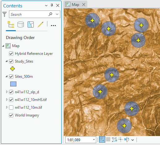
I changed the study site points to make them more visible and have blended the hillshade with a satellite image basemap:

Open the attribute table for the study sites.
Evaluate elevation and slope at each site
Calculate slope raster
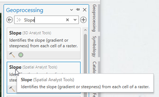
In the geoprocessing window (Analysis Tab > Tools) search for Slope.
Open the Spatial Analyst Slope tool.
Slope is calculated from elevations.
The input layer is therefore the DEM (not the hillshade!).
Why not calculate slope from the hillshade layer?
Because hillshade values (range 0-254) represent a color between white and black.
That’s it: colors.
Color values that describe a shade of gray.
Grayness doesn’t change as you go up or down slope, so the color isn't a direct function of elevation. (Look at a hillshade layer for proof.)
Grayness doesn’t change as slope gets steeper or flatter. Hillshade crayness is not a direct function of slope.
The grayness is a proxy for shadowing that is calculated by the location of a light source and the relationship of each location relative to that light source…
The location (altitude and angle) of the light source is determined by the user.
Therefore:
1. Don’t include hillshade values in a legend. This only advertises that you don't understand what hillshade values represent, and
2. Don't accidentally statistically summarize hillshade values while thinking you are working with values that correlate with elevation or slope.

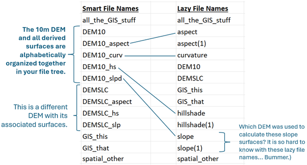
Notice in the tool setup that I have named the output to indicate the DEM from which the slope is being calculated. I added ‘slp’ for slope and ‘d’ for degrees. This is so the file name relates to the DEM at the root of all calculations made from it.
Organize alphabetically and happiness ensues.
In ArcGIS Pro, slope can be calculated in Degrees or Percent Rise.
Degrees is the standard slope angle you might be used to seeing.
Percent Rise is calculated from the standard practice units of rise over run or meter/meter. Rise over Run is multiplied by 100 to result in percent rise.
Meters/meter is not a unit for slope in ArcGIS Pro.
Calculate slope in degrees.
Leave the method as planar because at this scale and the efficient coordinate system assigned to the data, planar will perform accurate slope calculations.
Insert you should know box about planar versus geodesic calculations
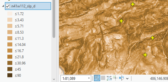
Inspect the results.
Question:
What is the range of slope values in the output slope raster?
Do these values seem logical for slope in degrees?
You now have an elevation raster surface and a slope raster surface.
Extract Values to Points
Identifythe elevation and slope values at the raster cell locations that intersect each study site point location.
Use a tool called Extract Values to Points.
This tool "extracts" the cell value at a point's location and creates a new field in the point's attribute table (usually called something like RASTERVALU). For each point, the corresponding raster value at the point's location is recorded in the point's attribute table.
You would need to run this tool twice, once for elevation and again for slope.
But wait!
Instead of running this tool twice, you can use a tool called Extract Multi-Values to Points and capture the elevation and slope for each point's location at the same time.

Notice:
- The tool modifies the input file. That is why you aren’t being asked to name an output. The only way to see the change is to open the attribute table for the Study Sites to see the new fields and data.
- I have added the DEM not the hillshade (because the DEM contains the actual elevation values, where the hillshade only contains values that represent shades of gray) and I’ve added the slope raster.
- The tool allows you to name the new columns, so you know what the values represent.
- I don’t have any of the points selected (tools only run on selected features).
Inspect the results in the attribute table.
Use the sort function to organize the attribute results and answer the following questions:
Round to the nearest integer.
USU students, use the "answer form" on Canvas to get immediate feedback on your results.
Buffer
The slope and elevation at the precise point location is interesting information, but might be too specific and misrepresentative of the area proximate to each XY point location.
Let's define an area around each point and evaluate the average elevation and slope within that area.
Use the Analysis “Buffer” tool to calculate a 500 meter circle centered around each point.
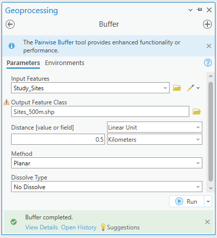
Inspect the results.
Get creative and think about what these buffer areas might represent: habitat areas, watersheds, riparian zones, census blocks, national park boundaries, counties, etc.
There are plenty of "areas" within which we might want to summarize raster values.
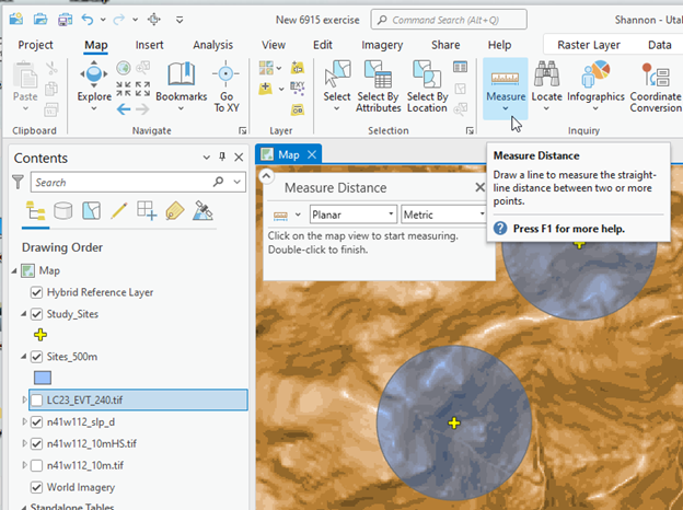
How can you verify that the areas are the correct size - that they were calculated correctly?
- Zoom in until you can see the individual buffer polygons.
- Use the Measure tool to measure the radius or diameter of one of the buffers and compare to your input buffer value.
Zonal Statistics
Zonal statistics is a tool designed to summarize raster cell values that fall within polygon zones of interest.
Calculate the minimum, maximum, and average slope within each buffer area. (This is really easy to do with the Zonal Statistics suite of tools).
Use the tool Zonal Statistics as a Table (Spatial Analyst) to summarize the elevation and slope values within each study site’s 500m area.
First, run Zonal Statistics as a Table for the Elevations.
Search for the tool and fill it out carefully.
Remember, this tool is designed to summarize the values of a raster within an ‘area of interest’ or ‘zone.’ The Zones are our study area buffers. The Value Raster is the Slope raster.
The output is a non-spatial table. It will add itself to the bottom of your contents pane.
Try to set up the tool on your own.
If you are unsure, think about it like this:
The Input Raster or Feature Zone Data is the Area of Interest. The key word is Zone:

The Input Value Raster is the raster that contains the values you want to summarize:
If you want to know the average elevations within each of the 500m buffer areas, you need to input the elevation raster (DEM).
![]()
If you want to know the average slopes of the 500m buffer areas, put in the slope raster.
Consider the different value rasters you could summarize: solar radiation, population densities, precipitation, temperatures, aspect, terrain roughness, etc.
The Zone Field options are fields within the Sites_500m attribute table. I chose ID because the ID field contains a unique value for each site. I want summary statistics for each individual site. If I wanted the summary statistics for the sites as a collective whole, I would create or find a field in the attribute table that contained a similar value for each site.
![]()
Calculate ALL Statistics Types.
The table will show up at the bottom of your contents pane.
Nothing will appear on the map as the table is not spatial.
Open the table and inspect the results.
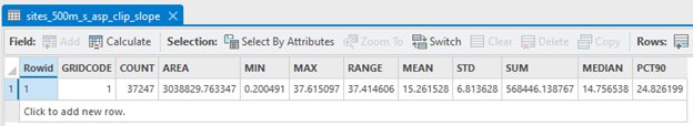
Decoding the Zonal Statistics
What exactly are we looking at, here?

Let's go through each field and think about what the results represent.
1. ID: This is the unique value used to identify each feature.
2. COUNT: The number of raster cells within each buffer zone.
Wait a minute!
Why are the areas different? Shouldn't they all be the same if the buffer areas areas all have 1000m diameters?
No, they shouldn't necessarily be the same.
Because the Site points aren't centered exactly in the middle of a given raster cell, the number of cells that fall within the 500m radius buffer area will vary. In our example, the count varies by 17 cells.
The buffer areas calculated from the polygon shapefile should be the same. But the number of raster cells selected by each buffer circle will differ.
In this image you can see the jagged edge of raster cells that intersect circle buffer areas.

3. AREA: These are calculated from the cell count and the area of a cell. The variability in area, while inconsistent, is a truer companion to the summary statistics because it reflects the actual area being summarized.
4. MIN: These are the lowest elevations found within each buffer area. What are the units of measure on these values? (You should know this.)
5. MAX: These are the highest elevations found within each buffer area.
6. RANGE: Naturally, these values are the difference between the min and max elevations.
7. MEAN: This is the average elevation of the cells intersecting each buffer area.
8. STD: Is the standard deviation of the mean values
This could be an interesting metric. For example, could the standard deviation of elevation be used as an indicator of elevation variation within each buffer area?...
9. SUM: This is the sum of all elevations within each buffer area. For elevation, this statistic doesn't really mean anything to us. But what if the cell values were house values or even binary true/false values... summing might produce a meaningful value.
10. MEDIAN: This is the "middle" value if all the elevations were ranked and listed in order.
11. PCT90: This is the 90th percentile value for the elevations within each buffer area. 90% of the buffer area's cell values fall below the value listed in this column.
Was that a lot?

Shake it off and keep moving.
Run Zonal Statistics as a Table on the Slope raster and answer the following questions.
Report with the correct units of measure and round to the nearest integer.
Congratulations!
Now you know how to summarize raster values within areas of interest.
Shifting gears to look at methods of clipping/cutting rasters using polygons.
Clipping versus Intersecting
Let’s dive deeper into understanding the characteristics of our study sites.
Now we want to summarize the slope characteristics for the parts of the study areas with southern exposures.
To do this, we will need the following map layers:
- Study area polygons (the 500m buffers)
- Slope raster layer (you calculated this earlier)
- Mapped areas of southern exposure (provided in the data folder)
Get your map cleaned up and set up.
Turn off the visibility of all data except for the data listed above.
Inspect the southern_aspects map layer.

- Ran the tool “Aspect” on the elevation raster (DEM).
- Classified the Aspect values into 3 classes
- Flat to East (-1 – 112.5 degrees)
- Southeast to Southwest (112.5 – 247.5 degrees)
- West to North (247.5 – 360 degrees)
- Ran Reclassify
- assigned the southern class (southeast to southwest) cells a new value of “1”
- Assigned the other two classes new cell values “NODATA”
- Ran “Raster to Polygon” to convert the southern facing cells to polygon areas.
The process we will work through is the same as before, using Zonal Statistics as a Table to summarize the slope raster. But first we need to limit the study area circles to just the areas that have been mapped as southern facing. We will do that using Clip and Intersect tools. There is a slight difference which you'll see with this demonstration.
Clip
Use the Clip tool (Analysis Tools) to cut the southern aspects layer with the circle buffers of the study site areas.
Use this diagram to set up the Clip tool.

Inspect the results by turning off the input data to verify that the southern features have been cut down to the study site buffer extents.
Open the attribute table for your southern site areas.
Notice that each polygon has a unique FID and Id, but share the same gridcode (“1”).
The gridcode is the value I assigned when reclassifying the south facing aspect cells.
Set up the Zonal Statistics as a Table tool to summarize the slopes of these southern aspect areas found within each study site area.
What are your choices for the Zone Field?

Stop and think about what your resulting summary statistics table will look like if you choose FID, Id, or gridcode.
How many zonal statistics table rows would you expect to produce if you use the FID field?
How many rows would you expect to produce if you used the gridcode field?
Run ZS as a Table using the gridcode field as your zone field.
Why only 1 row?
Because the gricode field is populated with only one unique value, so all polygons are being processed as one area.
But, we want to know the average slope of the southern facing cells for each individual study area.
We need our input zones to be uniquely identifiable – the attribute table needs to contain some record of which study site each polygon belongs to.
The study site designation is an attribute in the Sites_500m polygon shapefile.
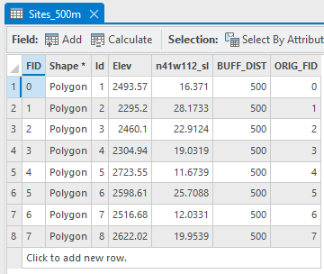
The FID, Id, and ORIG_FID fields all uniquely identify each study site buffer area.
Intersect
We can preserve and transfer the attributes of both the slope polygons and the study site buffer areas to the new ‘clipped’ output dataset by using the Intersect tool instead of the Clip tool.

Set up the Intersect tool with the southern_aspects and Sites_500m layers as input features. (Use the diagram as a guide.)
I named my output: Sites_500m_south_intersect
Run.
Inspect results by turning off visibility of input features.
Inspect attribute table.
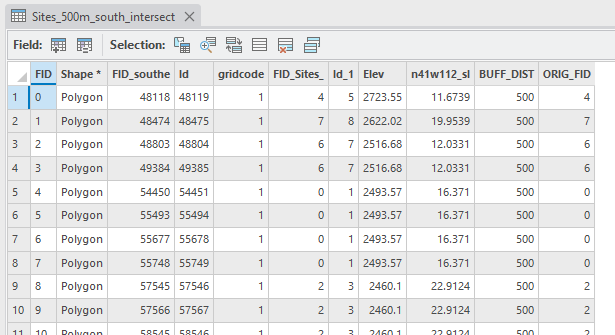
You should see fields containing the site FID, Id, and ORIG_FID values we wanted to preserve.
CHALLENGE
Run Zonal Statistics as a Table, but this time designate the field that will produce one set of slope summary statistics for each study site polygon. Then answer the following questions.
Of the 8 site areas, identify the site buffer area with the lowest mean slope for southern facing aspects and report the mean slope value.
Report with units of measure and round to the nearest integer.
Report the name from the Site_Name field.
You have successfully combined vector and raster data to analyze landscape characteristics of potenial study sites. These workflows and manipulations are very common and can be used to extract information from a wide variety of data types.
You have now mastered summarizing numeric raster data within zones of interest.