Vector Processing

The Basics:

You will use geoprocessing tools to spatially analyze global anti-shipping incidents (i.e. acts of piracy) within Exclusive Economic Zones.

“An Exclusive Economic Zone (EEZ) is a concept adopted at the Third United Nations Conference on the Law of the Sea (1982), whereby a coastal State assumes jurisdiction over the exploration and exploitation of marine resources in its adjacent section of the continental shelf, taken to be a band extending 200 miles from the shore.” - https://stats.oecd.org

Image: Curtis Suttle, 2016

Data:

• Anti-Shipping Activity Messages (ASAM) current through October 2018 (from the National Geospatial Intelligence-Agency: msi.nga.mil 05/22/19)
  • ASAM 11 Oct 18
• Exclusive Economic Zones (EEZ) (from marineregions.org)
  • World_EEZ_v8_2014_HR
• Countries (from Diva-GIS.org)
• Caribbean_Islands (from Diva-GIS.org)

 

 

Get Started:

Start a new ArcGIS Pro Map, and add your data.

1. Inspect the EEZ polygon. Dig into the data and familiarize yourself.

 

 

Look at the properties for the anti-shipping activity messages dataset (ASAM). Notice that the coordinate system is unknown.

Looking at the dataset in windows explorer shows us that the shapefile is made up of only

• the database file or attributes (*.dbf),
• the shapefile or geometry (*.shp), and
• the index file (*.shx).

 

 

Defining a Coordinate System

Every point of spatial data* must be assigned to a specific real world location by a set of coordinates. And, the pair of coordinate values relates to a coordinate system or spatial framework that is defined by three basic features: the datum (this is a model of the Earth’s curved surface), an origin (where are we going to start counting), and some unit of measure (feet, meters, degrees…).

If a dataset is missing its “projection” file** then you must define the data’s coordinate system before working with it in a GIS.

 

 

You cannot pick any old coordinate system you want for the data. The coordinate system must be one that relates to the coordinate values that define the locations. You might think you can find the coordinate values in the attribute table. For point data that would make very good sense. But it is not always the case. The easiest way to see these is from the “extent” section in the Properties of the dataset.

 

Again, extent is the north, south, west, and eastern-most points of the data. In this figure, the top value is 68ish “units” north of the horizontal origin for this dataset (it’s a positive value, so I’m assuming north).

There are no units (unknown) but the values are small, suggesting they are angles of latitude and longitude. This lets us know that we must assign a geographic coordinate system to this data. But which one? To us, the most common are North American Datum of 1983 (NAD 83) and the World Geodetic Survey of 1984 (WGS 84). Because it is a global dataset (piracy acts around the world), WGS 84 makes more sense. But fortunately for us, the website where we downloaded the data listed the coordinate system used. The coordinate system for the ASAM data is WGS84. WGS stands for World Geodetic Survey. It is a global dataset so a World coordinate system makes sense.

We will get way into coordinate systems next week. So hang in there. This is a great introduction to the concepts and importance of understanding these spatial frameworks.

Use the Define Projection tool to create a ‘projection file’ for this data.

1. Click on the Analysis tab in the top ribbon
2. Click on Tools and search “Define Projection”
3. Set your Input dataset to the ASAM data
4. Notice that you are not asked to name the output. This means the tool will overwrite and change the original file.
5. Set the Coordinate System to the geographic WGS 1984
6. Run

 

 

 

The result is somewhat underwhelming. Do you see any change? The change happened behind the scenes. The data displayed in your map now has a projection file associated with it. You can verify this by viewing the file in Windows File Explorer:

 

You should also verify the coordinate system in the layer’s properties.

 

Task 1: Identifying where the highest incident counts occur

In brief:

• Perform a Spatial Join to "count" how many Anti-Shipping incidents have happened in each offshore economic zone.
• Then normalize the count by the area of each EEZ to find the density.
  

Spatial joins

 

Determining where the incidents happened

First you will perform a Spatial Join to “count” how many Anti-Shipping incidents have happened in each EE Zone.

Then you will normalize the count by the area of each EE Zone.

1. On the Analysis tab, click "Tools" to open the Geoprocessing panel.

1. 1. Search for Spatial Join
   2. The 'Target Features' are the shapes within which you want to count.
      1. Set the Target Feature to the Economic Zones polygons
   3. The Join Features are the smaller geometry that you want to get a count of within your polygons
      1. Set the Join Features to the ASAM points.
   4. Set the Output Feature Class to your output folder and rename it EEZ_ASAM_SJ
      1. The output file will be the economic zone polygons with a count of the points saved into the attribute table.
      2. SJ to indicate the spatial join
   5. Join operation is one to one
   6. Set the Match Option to Intersect
      1. Because the points are discrete locations and each will either be inside or outside the polygon...
   7. Run

Go to the Attributes Table of the newly created layer and verify there is a field containing the count of points falling within each polygon.

How can you find out which zone has the highest number of piracy points falling within it?

Mua ha ha. Not a rhetorical question.

 

 

 

Task 2: Determining areas with high density of incidents

Normalizing by area

 

Bigger areas might be more likely to have more piracy points. Smaller areas might have many ASAM points, but not seem like a lot because the area is so small. We can account for the differences in area by normalizing the data. To normalize the data, you will divide the count of incidents by the area of each EEZ. This will result in the density of piracy acts with standardized units instead of relying on a raw count per zone.

Calculations can be made in the attribute table using the field calculator. This tool allows you to divide, add, subtract, multiply between fields (among other functions).

You’ve done this before with the population density of Census Blocks.

You will run the field calculator to divide the two fields but first you need a new empty field to store the result of your division. While you are at it, you should probably calculate the area (geometry) so you know the area units are square miles.

1. In the attribute table of your new spatially joined polygon data, add a field

1. 1. Name it Inc_km2 (Incidents per square kilometer)
   2. Set the Data Type to Float

2. Create and populate a new Area field in the EEZ_ASAM_SJ layer

1. 1. Name it Area_km2 (Area in kilometer squared)
   2. Set Data Type to Float
   3. Right click the new field header and calculate geometry
   4. Set the Property to Area (Geodesic)
   5. Set the Area Unit to square kilometers
   6. Set the coordinate system to match the ASAM points
   7. Run (this may take a hot minute)

3. Perform a field calculation into the Inc_km2 field (your density field)

1. 1. Right click the field/column header
   2. Divide the Join_Count field by the Area_km2
   3. run

Don't type or copy paste into the formula field.
Double click on field names and math symbols to add to formula field.

 

 

Task 3: Determine how many incidents occured near the US?

Select by location

 

This is a tool that lets you select features from a dataset based on their spatial proximity to another dataset. For example, you can use this tool to select ASAM points that are ‘within a distance of’ the US polygon shapefile.

1. Select the ‘United States’ record from the Countries layer.
   • Either from the attribute table
   • click on it using the “select elements” tool 

Open the Select by Location tool:

 

Think carefully about how this tool works.

Read the window like this:

Select features from a layer (we want to select and count the ASAM points near the US - so input the ASAM points)

that are within a distance (200 nautical miles) of (selection method)

the source layer (which is the countries shapefile)

You have selected the US, so it will only run on the US polygon from the Countries shapefile.

 

Don’t try to manually count these as often times points are stacked on top of one another.

Where can you see how many points or records are selected? ArcGIS counts them for you…

 

Task 4: Determine the number of Piracy acts happened in the Caribbean

Buffer and Clip

 

In this task you will learn how to Buffer (create a ‘balloon’ around) the island polygons and use that buffer to Clip (or cut) the piracy points to both isolate the points within 100 nautical miles and to visualize the results for a formal map.

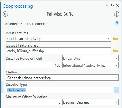
1. Create a 100 nautical mile buffer around the Caribbean_Islands layer
   1. Search for the Pairwise Buffer Tool
      1. Set the Input feature (the islands)
      2. Make sure the output file is being sent to your Output folder
      3. Name it something that accurately represents the new layer being created
      4. Set the buffer distance and units
      5. Set the Dissolve type to ALL
         1. This merges the overlapping buffers into one smooth shape

 

 

Verify the results.

You may find that there are some points falling within the island polygons:

This could be an error in the coordinate values, or maybe inland waters?

 

1. Use the Buffer shapefile to Clip the ASAM data
   1. Search for the Clip tool
   2. Use the tool to help guide your inputs
      1. Input Features are the things that will be clipped
      2. Clip Features are the shapes to define the area to be clipped
   3. You may want to name the output something like, IDK, “Pirates of the Caribbean”…
   4. Leave the XY Tolerance blank
   5. Run

 

 

Results should look something like this:

 

 

We specify "shapefile" to remind you that this is spatial data. The Caribbean Island polygons are rigidly defined areas that may or may not align with the exact border of each island or country. It also may or may not include the correct area defined as "the Caribbean Islands." And the incident locations may or may not be as exact as the coordinate values indicate they are. And this data is temporal in nature (collected and reflecting a certain time period that may or may not be up to date).

Therefore, when you state your results, keep these things in mind when reporting or using your results. Your results are a best estimate given the accuracy and precision of the data.

 

 

Prepare a Formal Map Figure for Submission:

 

Map’s Purpose: to display the Anti-Shipping points within 100 nautical miles of the Islands of the Caribbean.

• Include date of record
• Author and Data Credits
• Other map elements needed to support map purpose
• Remove basemap credits
• Exported as high resolution image (not a screenshot)

 

ArcGIS Online has a wide variety of different basemaps you can use.

Access ArcGIS Online from the Add Data button instead of the Basemaps button.

 

Example Maps:

 

View other submission details on the assignment's Canvas page.