HT Errors

Errors in Hypothesis Testing

When conducting a hypothesis test, a researcher either rejects or fails to reject the null hypothesis. If they reject a false null hypothesis or fail to reject a true one, they are, of course, correct. However, when they reject a true null hypothesis or fail to reject a false one, they have made an error. These errors are called Type I and Type II errors respectively and are important to the process of hypothesis testing.

Type I Error: Reject a null hypothesis when it is true.

Type II Error: Fail to reject a null hypothesis when it is false.

Diagram showing a 2×2 table labeled “Truth” across the top and “Choice” along the left side. The top row represents choosing the null hypothesis (H₀), and the bottom row represents choosing the alternative hypothesis (Hₐ). When H₀ is true and chosen, the result is labeled “Correct.” When H₀ is true but Hₐ is chosen, it’s labeled “Type I Error.” When Hₐ is true and H₀ is chosen, it’s labeled “Type II Error.” When Hₐ is true and chosen, it’s labeled “Correct.” Type I Error and Type II Error cells are shaded orange.

Null and Alternative Distributions of the Sample Mean

Consider drawing from a population with unknown mean and variance $\sigma^2$. The distribution of the sample mean is normal if the sample size is large or the population distribution is normal.

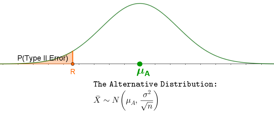
The sample mean is an unbiased estimator of the population mean. Thus if $H_0=\mu = \mu_0$ is true, $E(\bar{X})=\mu_0$ and $\small{\bar{X}\sim N\left(\mu_0,\frac{\sigma^2}{n}\right)}$. If the $\mu = \mu_A$ instead, $E(\bar{X}) = \mu_A$ and $\small{\bar{X}\sim N\left(\mu_A,\frac{\sigma^2}{n}\right)}$.

$Chart titled “The Distribution of X̄.” It shows two overlapping bell curves representing sampling distributions. The left curve, in purple, is labeled “μ₀” and represents the null distribution ( \bar{X} \sim N(\mu_0, \frac{\sigma^2}{\sqrt{n}}) ). The right curve, in green, is labeled “μₐ” and represents the alternative distribution ( \bar{X} \sim N(\mu_A, \frac{\sigma^2}{\sqrt{n}}) ). The purple and green points on the horizontal axis mark the centers of the two distributions, illustrating how the means differ under the null and alternative hypotheses.$

It is possible to use these distributions to find the probabilities of making Type I or Type II errors.

The Probability of a Type I Error

The probability of a Type I error, denoted $\alpha$, is the probability that a null hypothesis is rejected when it is true.

If the null hypothesis is true, the distribution of the sample mean is centered at $\mu_0$. Consider rejecting the null hypothesis when the value of the sample mean is greater than some value R. The probability of a type I error is the probability under the null distribution that the sample mean is greater than R.

$Bell curve titled “The Null Distribution.” The purple curve represents the sampling distribution of the sample mean under the null hypothesis, centered at μ₀. A vertical line at point R marks the rejection region on the right tail, shaded orange, labeled “P(Type I Error).” The formula below reads ( \bar{X} \sim N(\mu_0, \frac{\sigma^2}{\sqrt{n}}) ), indicating the sampling distribution of the mean under the null hypothesis.$

The Probability of a Type II Error and Power

The probability of a Type II error, denoted $\beta$, is the probability that a null hypothesis is not rejected when it is false.

If the null hypothesis is false, the distribution of the sample mean is centered at $\mu_A$. If we fail to reject the null hypothesis when the value of the sample mean is less than R, then the probability of a Type II error is the probability under the alternative distribution that the sample mean is less than R.

$Bell curve titled “The Alternative Distribution.” The green curve represents the sampling distribution of the sample mean under the alternative hypothesis, centered at μₐ. A vertical line at point R on the left marks the rejection region, shaded orange and labeled “P(Type II Error).” The formula below reads ( \bar{X} \sim N(\mu_A, \frac{\sigma^2}{\sqrt{n}}) ), indicating the sampling distribution of the mean when the alternative hypothesis is true.$

To compute the probability of a Type II error, a specific value must be stated in the alternative hypothesis.

The power of a test is the probability that the null hypothesis is correctly rejected, that is, it is rejected when it is false.

The power, of a hypothesis test is the probability that the null hypothesis is rejected when it is false.

Continuing the example and rejecting the null hypothesis when the sample mean is greater than R, the power is the probability under the alternative hypothesis that the sample mean is greater than R.

The power is equal to 1 - P(Type II error).

$Bell curve titled “The Alternative Distribution.” The green curve represents the sampling distribution of the sample mean under the alternative hypothesis, centered at μₐ. The region to the right of point R is shaded orange and labeled “Power,” representing the probability of correctly rejecting the null hypothesis. Below, the formula ( \bar{X} \sim N(\mu_A, \frac{\sigma^2}{\sqrt{n}}) ) describes the sampling distribution under the alternative hypothesis.$

Power = 1 - P(Type II Error)

Like the probability of a Type II Error, a specific alternative value must be specified to compute power.

Errors in Hypothesis Testing Applet

Use the applet to investigate type I and type II errors for the simple hypotheses given. The rejection region, null and alternative mean values, and standard deviation can be adjusted. You can choose whether or not to see the alternative hypothesis and related probabilities.

Computing P(Type II Error) and Power in Practice

The way we framed the hypothesis test in the above discussion is useful for understanding Type I and Type II errors. In practice, however,

The population variance, $\sigma^2$, is generally unknown and has to be estimated from the data with $S^2$.
The usual form of the test statistic is a standardized mean, $\frac{\bar{X}-\mu_0}{s/\sqrt{n}}$ rather than the sample mean itself.

Thus we use the t-distribution to find the probabilities of the Type I and Type II Errors.

For a test that rejects the null hypothesis for a value of the sample mean greater than R:

P(Type I Error) = $P\left(\frac{\bar{X}-\mu_0}{s/\sqrt{n}}> \frac{R-\mu_0}{s/\sqrt{n}}\right)$
P(Type II Error) = $P\left(\frac{\bar{X}-\mu_A}{s/\sqrt{n}} \lt \frac{R-\mu_A}{s/\sqrt{n}}\right)$

Example: Movie Length

Is the mean length, $\mu$, of a Netflix movie 90 minutes or 120 minutes?

Find the rejection region if P(Type I error) = 0.05.

For the movie length data, the sample standard deviation s = 18 and the sample size n = 32.

Since 120 is greater than 90, reject the null hypothesis for some large value, R, of the sample mean. That is, reject for R such that P(Type I Error) = $P\left(\frac{\bar{X}-90}{18/\sqrt{32}}> \frac{R-90}{18/\sqrt{32}}\right) = 0.05$ $Normal distribution curve shown in purple, centered at zero with x-axis values ranging from -3.5 to 3.5. The right tail beyond approximately 1.7 is shaded purple, representing an area of 0.05. A label points to the shaded region with “0.05,” indicating the significance level (α). The boundary of the shaded region is marked at ( \frac{R - 90}{18 / \sqrt{32}} ), showing the critical value for a right-tailed hypothesis test.$ The 95th percentile of a $t_{31}$ distribution is 1.70 so \[\frac{R-90}{18/\sqrt{32}} = 1.70\] and R = 95.40.

If R = 95.40 minutes and we reject for $\bar{X}>R$, $\alpha$ = 0.05.

Example: Movie Length

Is the mean length, $\mu$, of a Netflix movie 90 minutes or 120 minutes?

Find P(Type I error) if the test rejects for $\bar{X}$ > 100 minutes.

For the movie length data, the sample standard deviation s = 18 and the sample size n = 32.

$\begin{array}{lrc}P(\verb"Type Error") & = & P\left(\frac{\bar{X}-90}{18/\sqrt{32}} > \frac{100-90}{18/\sqrt{32}}\right)\\ & = & P(T > 3.14)\\ & = & 0.002\end{array} $

Thus, if the true mean is 90 minutes and the test rejects for $\bar{X}>100$, P(Type I Error) = 0.002.

Example: Movie Length

Is the mean length, $\mu$, of a Netflix movie 90 minutes or 120 minutes?

Find P(Type II error) if the test rejects for $\bar{X}$ > 100 minutes.

For the movie length data, the sample standard deviation s = 18 and the sample size n = 32.

$\begin{array}{lrc}P(\verb"Type II Error") & = & P\left(\frac{\bar{X}-120}{18/\sqrt{32}} \lt \frac{100-120}{18/\sqrt{32}}\right)\\ & = & P(T \lt -6.29)\\ & \approx & 0\end{array} $ Thus, if the true mean is 120 minutes and given the standard error, there's virtually no chance of obtaining a mean less than 95.

The power for this test is about 100%.