- When drawing 2 balls from the jar, there can be 0 red balls, 1 red ball, or 2 red balls. The sample space for X is
S = {0,1,2}. Use the tree diagram to find the probabilities of each.:

The probability of drawing 2 red balls is 3/10, the probability of drawing 1 red ball is 3/10+3/10 = 3/5, and the probability of drawing 0 red balls is 1/10. This produces the probability mass function shown.
- P(X ≤ 1) = P(X = 0) + P(X = 1) = 1/10 + 3/5 = 7/10.
Or: P(X ≤ 1) = 1 - P(X = 2) = 1 - 3/10 = 7/10. - P(X ≤ 0) 1/10.
P(X ≤ 1) = P(X = 0) + P(X = 1) = 1/10 + 3/5 = 7/10.
P(X ≤ 2) = P(X = 0) + P(X = 1) + P(X = 1) = 1/10 + 3/5 +3/10 = 1.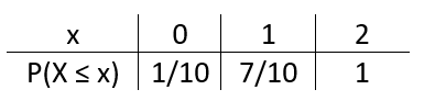
- From the cdf table, P(X ≤ 1) = 7/10
Discrete Random Variables
Colorblindness is caused by a
recessive gene on the X chromosome. Since men have only one X chromosome, if
a man carries the colorblindness allele (gene form), he will have the trait. Women have two X chromosomes so, for a woman to be colorblind, she must
inherit the allele from both parents. Suppose both parents carry one colorblindness allele. Let X (pun intended!) denote the number of
colorblindness alleles their daughter inherits. X is a discrete random variable.
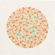
Click on the picture to take the Ishihara test for colorblindness.
A discrete random variable maps the outcomes of a chance process to a countable set of numbers. Variables corresponding to outcomes that are are counted are discrete. Values might be fractional and there might be infinite possibilities, however, between any two observable values there is a gap.
A woman can inherit 0, 1, or 2 of the allese for colorblindness from her parents. Let X be a random variable that indicates the number of alleles a randomly chosen woman inherits from parents who are both carriers.
X is always 0, 1, or 2. There cannot be 0.5 or 1.7 inherited alleles.
X is a discrete random variable.
The Distribution of a Discrete Random Variable
Tables, graphs, and formulas can describe the distribution of a discrete random variable. These indicate the possible values of the random variable along with the associated probabilities. It is sometimes useful to state specific probabilities, and sometimes cumulative probabilities.
The tables and graphs below all contain the same information, the distribution of X, the number of alleles for colorblindness carried by a daughter of two carriers of the colorblindness allele.
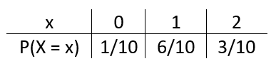
In Table 1 and Graph 1, the possible values are indicated along with the probabilities of observing those values exactly. This is called the Probability Mass Function (pmf).
Notice that probability is associated with the values 0, 1, and 2 only.
In Table 2 and Graph 2, the possible values of the random variable are indicated along with the probabilities of observing a value no greater than the indicated value. This is the Cumulative Distribution Function (cdf).


In Table 2 and Graph 2, the possible values of the random variable are indicated along with the probabilities of observing a value no greater than the indicated value. This is the Cumulative Distribution Function (cdf).
A function that indicates the observable values of a discrete random variable and their associated probabilities is called a probability mass function. A function that indicates the observable values of a discrete random variable and associated cumulative probabilities is called the cumulative distribution function.
The Probability Mass Function
The probability mass function (pmf) describes the distribution of a discrete random variable in terms of the possible outcomes and the specific associated probabilities. The pmf can be given as a table, a graph, or a formula.
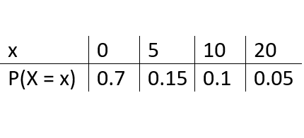
Consider a raffle of 20 tickets. 6 tickets are drawn for prizes. The one first prize winner gets $\$20$, 2 second prize winners get $\$10$, and three third prize winners get $\$5$. Let X denote the amount of money a person could win with a raffle ticket. The table and the graph display the probability mass function of X.
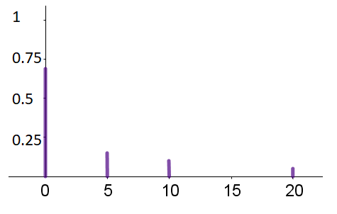
$\rightarrow$ The probability mass function of a discrete random variable indicates the possible values of the random variable and the probabilities of observing those values.
NOTATION
The probability mass function is denoted as 'P(X = x)' or just 'P(x)'.
The probability mass function is denoted as 'P(X = x)' or just 'P(x)'.
The probability mass function for X, the number of alleles for colorblindness carried by a daughter of two carriers of the colorblindness allele, is shown in the table and the graph.


All the values that the random variable can assume are identified in probability mass function. The probability associated with a value other than these is 0. The sum of the probabilities is 1.
For a discrete random variable, X, with values x or x1,x2...xn
- All probabilities are between 0 and 1: $\small{0 \leq P(X=x_i) \leq 1}$.
- The sum of the probabilities of all outcomes is 1: $\small{\sum_{i=1}^nP(X=x_i) = 1}$.
The Cumulative Distribution Function
The cumulative distribution function (cdf) describes the distribution of a discrete random variable in terms of the possible outcomes and the associated cumulative probabilities. A cumulative probability indicates that probability that the random variable takes on a value no larger than the corresponding value. The cdf can be given as a table, a graph, or a formula.
Consider a raffle of 20 tickets. 6 tickets are drawn for prizes. The one first prize winner gets $\$20$, 2 second prize winners get $\$10$, and three third prize winners get $\$5$. Let X denote the amount of money a person could win with a raffle ticket. The table and graph display the cumulative distribution function of X.

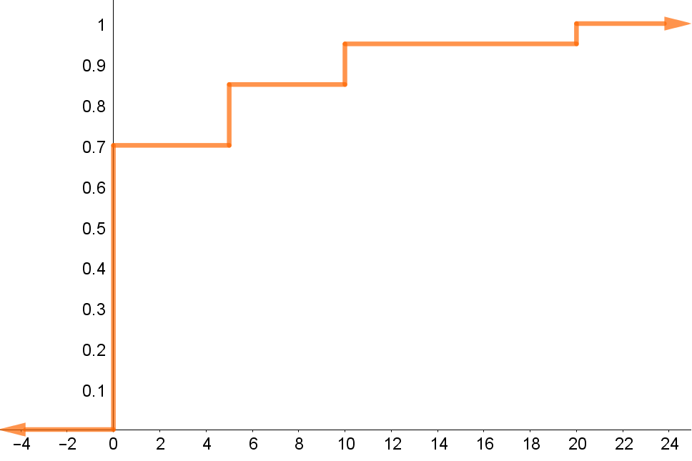
$\rightarrow$ The cumulative distribution function of a discrete random variable indicates each of the possible values of the random variable, and the probability of observing anything equal to or less than each of the values.
NOTATION
The cumulative distribution function for a discrete random variable is denoted as 'P(X ≤ x)'.
The cumulative distribution function for a discrete random variable is denoted as 'P(X ≤ x)'.
The cumulative distribution function for X, the number of alleles for colorblindness carried by a daughter of two carriers of the colorblindness allele, is shown in the table and the graph.

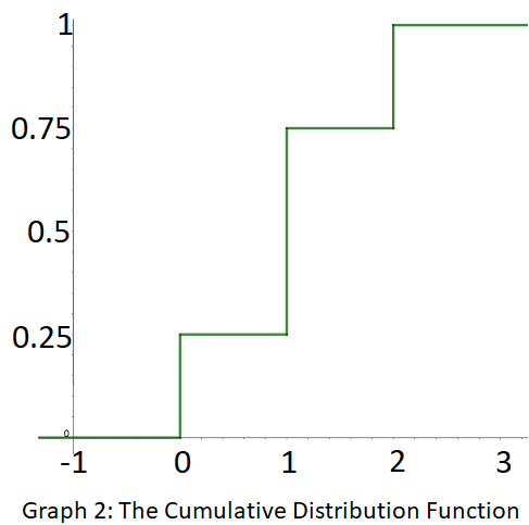
The cumulative distribution function is 0 for any value less than the smallest observable value (0 in this case). In other words, there
is no probability that a value less than the smallest possible value would be observed.
The cdf increases only at the locations of the possible values and does not decrease. Between observable values, the cdf is constant. The
random variable in this example can only assume the values 0, 1, and 2. Thus P(X ≤ 1) = P(X = 0) + P(X = 1). P(X ≤ 1.5) = P(X = 0) + P(X = 1)
as well since 0 and 1 are the only observable values that are less than 1.5.
The probability that the random variable is less than or equal to 2 is 1 since 0, 1, and 2
are all less than or equal to 2. For any value x that is greater than 2, P(X \leq x) = 1 since 0, 1, and 2 are all less than that value.
Properties of the cumulative distribution function with minimum value L and maximum U:
- If x is less than L, the cdf evaluated a x is 0.
- If $\small{a}$ and $\small{b}$ are two values such that $\small{a < b}$ then $\small{P(X \leq a) \leq P(X \leq b)}$. (The cdf is non-decreasing.)
- If x is greater than U, the cdf evaluated a x is 1.